A reliability program plan is used to document exactly what “best practices” (tasks, methods, tools, analysis and tests) are required for a particular (sub)system, as well as clarify customer requirements for reliability assessment. For large scale, complex systems, the reliability program plan should be a separate document. Resource determination for manpower and budgets for testing and other tasks is critical for a successful program. In general, the amount of work required for an effective program for complex systems is large.
A reliability program plan is essential for achieving high levels of reliability, testability, maintainability and the resulting system Availability and is developed early during system development and refined over the systems life-cycle. It specifies not only what the reliability professional does, but also the tasks performed by other stakeholders. A reliability program plan is approved by top program management, which is responsible for allocation of sufficient resources for its implementation.
A reliability program plan may also be used to evaluate and improve availability of a system by the strategy on focusing on increasing testability & maintainability and not on reliability. Improving maintainability is generally easier than reliability. Maintainability estimates (Repair rates) are also generally more accurate. However, because the uncertainties in the reliability estimates are in most cases very large, it is likely to dominate the availability (prediction uncertainty) problem; even in the case maintainability levels are very high. When reliability is not under control more complicated issues may arise, like manpower (maintainers / customer service capability) shortage, spare part availability, logistic delays, lack of repair facilities, extensive retro-fit and complex configuration management costs and others. The problem of unreliability may be increased also due to the “domino effect” of maintenance induced failures after repairs. Only focusing on maintainability is therefore not enough. If failures are prevented, none of the others are of any importance and therefore reliability is generally regarded as the most important part of availability. Reliability needs to be evaluated and improved related to both availability and the cost of ownership (due to cost of spare parts, maintenance man-hours, transport costs, storage cost, part obsolete risks, etc.). But, as GM and Toyota have belatedly discovered, TCO also includes the down-stream liability costs when reliability calculations do not sufficiently or accurately address customers’ personal bodily risks. Often a trade-off is needed between the two. There might be a maximum ratio between availability and cost of ownership. Testability of a system should also be addressed in the plan as this is the link between reliability and maintainability. The maintenance strategy can influence the reliability of a system (e.g. by preventive and/or predictive maintenance), although it can never bring it above the inherent reliability.
Elements of creating and supporting a reliability program
The basic elements of creating and supporting a reliability program.
Gather Requirements and Set Reliability Goals – Reliability Goals start with understanding customer needs and the competitive situation surrounding those needs. However, this information must also be viewed through the lens of marketing strategy. Setting a new standard in reliability is a proven way to gain market share. Low warranty costs may also allow a lower price than the competition. Reliability Goals for complex products have at least two dimensions: how frequently will random-in-time failures be tolerated, and how long the device must last.
The first of these is usually expressed as a failure rate (e.g. Annual Failure Rate, or AFR, in % per year) when speaking to customers, or as a Mean Time Between Failures (MTBF) when speaking to engineers. The second of these is often expressed as the L1, L10, or L50 life, when 1%, 10%, or 50% of the devices, respectively, have failed in an end-of-life (wear-out) failure mode. The latter can be expressed in time (hours or months), number of cycles, takeoffs plus landings, sorties, and so on (e.g., L10 = 1000 cycles).
These two dimensions of reliability are independent. It is possible to have an MTBF of millions of hours, a situation where random-in-time failures are rare, yet have most units fail before five years because certain components inevitably wear out. Subassemblies and components that have wear-out failure modes which cannot economically be pushed to last long enough are often called “service items.” Examples are rechargeable batteries and automobile tires.
Sometimes these service items can be incorporated with a consumable item or grouped with other service items in logical periodic replacement cartridges. Examples are putting the drum of a laser printer in the cartridge with the powdered ink, or selling defibrillator pads with battery packs for periodic replacement.
Indeed, service strategy is one of the major inputs to the product design. Sometimes sterility considerations or shelf life make it logical to break the product into a long-lived portion and a “disposable” portion. An example of this is an electronic thermometer with a disposable sheath for each use. Other considerations from the service plan may be to design a low cost, unserviceable, sealed unit, or to perform on-site repairs due to size. If the intention is to use loaners units and bring all units to one centralized location for repair, the device must be rugged enough for multiple shipments.
Risk Control Measures (mitigations) from Risk Management (safety) are another rich source of Reliability Goals. Safety may dictate an architectural change to the product to achieve desired reliability. An example of this is the dual-diagonal braking system on automobiles, which is now standard. Other sources of Reliability Goals are external standards (e.g. ISO, IEC) and the manufacturing plan. For example, if manufacturing screening is to be utilized, good design margin is needed to ensure the product’s fatigue life will be only slightly consumed during manufacturing.
Product Design – Product design is the process of creating a new product to be sold by a business to its customers. A very broad concept, it is essentially the efficient and effective generation and development of ideas through a process that leads to new products.
Process Design – The activity of determining the workflow, equipment needs, and implementation requirements for a particular process. Process design typically uses a number of tools including flowcharting, process simulation software, and scale models.
Allocate Reliability Goals to Subassemblies and Key Components – If the product contains redundancy or the ability to partially function in the presence of failures, a Reliability Block Diagram should be constructed showing how the reliability of each individual piece combine to produce the top-level reliability. Based on field experience with previous models, competitive information, and engineering judgment, the top-level goal for random-in-time failures should be allocated to subassemblies and key components. This will typically result in a Pareto of (unequal) individual failure rates.
Validation and verification – As either prototypes or the first production pieces become available, the reliability program must facilitate tests that are conducted to validate that the reliability requirements do indeed produce the desired product reliability. When these requirements have been validated it is necessary to verify that the production processes can produce products that meet these requirements.
Develop Analytical Models and Reliability Predictions – Depending on the nature of each key component or subassembly, develop an estimate of reliability based on: Finite Element Analysis (FEA), comparison to similar designs, Physics of Failure (PoF), parts count prediction techniques, and supplier test data. Be cautious, however, when using supplier data. If your application is more stressful than the conditions of the supplier test, additional testing will be necessary.
By comparing the allocated Reliability Goal with the various analytical models or reliability predictions for each subassembly or key component, one can see where to focus the reliability engineering effort. It may be possible to re-allocate the individual goals in light of the analytical results. If the gap is large, an architectural change in the product, such as specifically targeted redundancy, should be considered.
Begin Long Term Life Tests – Often called “cycle testing,” this is subjecting components which rotate, flex, or receive repetitive electrical or mechanical stresses to several worst case lifetimes of wear. Depending on the product’s intended usage pattern, it may be possible to accomplish this quickly by increasing the frequency of cycling. For example, switches, cables, and connectors can usually be thoroughly tested over a weekend. But if the component is intended to run 24/7, such as a disk drive’s spindle, it may require an Accelerated Life Test (ALT) where the stress is increased, to see the relevant failure modes.
Whether the frequency or the stress or both are increased, the goal is to discover relevant failures. It is possible to miss failure modes because some things only happen over time and don’t speed up with cycles. An example of this would be copper migration and subsequent oxidation in a connector. It is also possible to produce “foolish failures” which will not occur in the customer environment. These are test artifacts, which result from the accelerating stress. Reliability engineering requires experience and judgment.
Wear-out failure modes are improved by identifying the “reservoir” of material that is being consumed (or transformed) by a “process.” One then increases the reservoir and / or slows down the process to push out the occurrence of failure until satisfactory life is achieved. If this is not possible, preventive maintenance is used to restore the reservoir of material by replacing a service item.
Post-production evaluation. The reliability program must make provisions for collecting and analyzing data from products during their useful life by taking random samples, customer feedback and from the warranty records as well.
The reliability plan should clearly provide a strategy for availability control. Whether only availability or also cost of ownership is more important depends on the use of the system. For example, a system that is a critical link in a production system – e.g. a big oil platform – is normally allowed to have a very high cost of ownership if this translates to even a minor increase in availability, as the unavailability of the platform results in a massive loss of revenue which can easily exceed the high cost of ownership.
The mean life of a product is the average time to failure of identical products operating under identical conditions. Mean life is also referred to as the expected time to failure. Mean life is denoted by mean time to failure (MTTF) for nonrepairable products and mean time between failures (MTBF) for repairable products. The reliability professional should exercise care in the use of the terms MTBF and MTTF.
Mean time between failures (MTBF) describes the expected time between two failures for a repairable system, while mean time to failure (MTTF) denotes the expected time to failure for a non-repairable system. For example, three identical systems starting to function properly at time 0 are working until all of them fail. The first system failed at 100 hours, the second failed at 120 hours and the third failed at 130 hours. The MTBF of the system is the average of the three failure times, which is 116.667 hours. If the systems are non-repairable, then their MTTF would be 116.667 hours.
In general, MTBF is the “up-time” between two failure states of a repairable system during operation as outlined here:
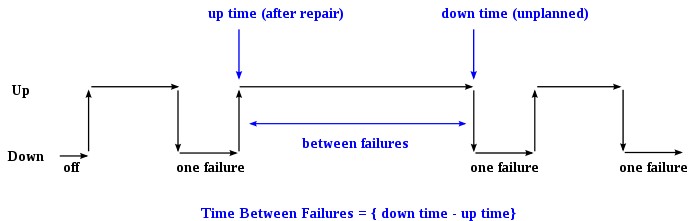
For each observation, the “down time” is the instantaneous time it went down, which is after (i.e. greater than) the moment it went up, the “up time”. The difference (“down time” minus “up time”) is the amount of time it was operating between these two events.
Once the MTBF of a system is known, the probability that any one particular system will be operational at time equal to the MTBF can be calculated. This calculation requires that the system is working within its “useful life period”, which is characterized by a relatively constant failure rate (the middle part of the “bathtub curve”) when only random failures are occurring. Under this assumption, any one particular system will survive to its calculated MTBF with a probability of 36.8% (i.e., it will fail before with a probability of 63.2%). The same applies to the MTTF of a system working within this time period.
MTBF value prediction is an important element in the development of products. However, it is incorrect to extrapolate MTBF to give an estimate of the life time of a component, which will typically be much less than suggested by the original MTBF due to the much higher failure rates in the “end-of-life wearout” part of the “bathtub curve”.
Reliability engineers and design engineers often use reliability software to calculate a product’s MTBF according to various methods and standards (MIL-HDBK-217F, Telcordia SR332, Siemens Norm, FIDES,UTE 80-810 (RDF2000), etc.). However, these “prediction” methods are not intended to reflect fielded MTBF as is commonly believed; the intent of these tools is to focus design efforts on the weak links in the design.
By referring to the figure above, the MTBF is the sum of the operational periods divided by the number of observed failures. If the “Down time” (with space) refers to the start of “downtime” (without space) and “up time” (with space) refers to the start of “uptime” (without space), the formula will be.

The MTBF is often denoted by the Greek letter θ, or

The MTBF can be defined in terms of the expected value of the density function ƒ(t)
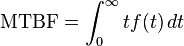
where ƒ is the density function of time until failure – satisfying the standard requirement of density functions –
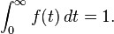
In this context (of reliability) is density function ƒ(t) also often referred as reliability function R(t).
There are many variations of MTBF, such as mean time between system aborts (MTBSA) or mean time between critical failures (MTBCF) or mean time between unscheduled removal (MTBUR). Such nomenclature is used when it is desirable to differentiate among types of failures, such as critical and non-critical failures. For example, in an automobile, the failure of the FM radio does not prevent the primary operation of the vehicle. Mean time to failure (MTTF) is sometimes used instead of MTBF in cases where a system is replaced after a failure, since MTBF denotes time between failures in a system which is repaired. MTTFd is an extension of MTTF, where MTTFd is only concerned about failures which would result in a dangerous condition.
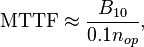
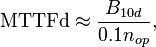
where B10 is the number of operations that a device will operate prior to 10% of a sample of those devices would fail. B10d is the same calculation, but where 10% of the sample would fail to danger. nop is the number of operations/cycles.
MTBF Example
If “λ” is the number of failures per hour, the MTBF is expressed in hours.
A system has 4000 components with a failure rate of 0.02% per 1000 hours. Calculate λ and MTBF.
λ = (0.02 / 100) * (1 / 1000) * 4000 = 8 * 10-4 failures/hour
MTBF = 1 / (8 * 10-4 ) = 1250 hours
Failure rate
It is the reciprocal of the mean life. Failure rate is usually denoted by the letter f or the Greek letter lambda (λ).
Availability
The term availability has the following meanings
- The degree to which a system, subsystem or equipment is in a specified operable and committable state at the start of a mission, when the mission is called for at an unknown, i.e. a random, time. Simply put, availability is the proportion of time a system is in a functioning condition. This is often described as a mission capable rate. Mathematically, this is expressed as 100% minus unavailability.
- The ratio of (a) the total time a functional unit is capable of being used during a given interval to (b) the length of the interval.
For example, a unit that is capable of being used 100 hours per week (168 hours) would have an availability of 100/168. However, typical availability values are specified in decimal (such as 0.9998). In high availability applications, a metric known as nines, corresponding to the number of nines following the decimal point, is used. With this convention, “five nines” equals 0.99999 (or 99.999%) availability.
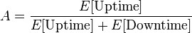
The most simple representation for availability is as a ratio of the expected value of the uptime of a system to the aggregate of the expected values of up and down time, or
If we define the status function X(t) as
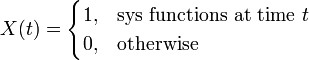
therefore, the availability A(t) at time t>0 is represented by

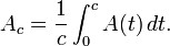
Average availability must be defined on an interval of the real line. If we consider an arbitrary constant c>0, then average availability is represented as
Limiting (or steady-state) availability is represented by
Limiting average availability is also defined on an interval [0,c] as,
Availability is the probability that an item will be in an operable and commitable state at the start of a mission when the mission is called for at a random time, and is generally defined as uptime divided by total time (uptime plus downtime).
Availability Example
If we are using equipment which has a mean time to failure (MTTF) of 81.5 years and mean time to repair (MTTR) of 1 hour:
MTTF in hours = 81.5*365*24=713940 (This is a reliability parameter and often has a high level of uncertainty!)
Inherent Availability (Ai) = MTTF/(MTTF+MTTR) = 713940/713941 =99.999859%
Inherent Unavailability = 0.000141%
Outage due to equipment in hours per year = 1/rate = 1/MTTF = 0.01235 hours per year.
Maintainability
Maintainability is defined as the probability of performing a successful repair action within a given time. In other words, maintainability measures the ease and speed with which a system can be restored to operational status after a failure occurs. This is similar to system reliability analysis except that the random variable of interest in maintainability analysis is time-to-repair rather than time-to-failure. For example, if it is said that a particular component has a 90% maintainability for one hour, this means that there is a 90% probability that the component will be repaired within an hour. When you combine system maintainability analysis with system reliability analysis, you can obtain many useful results concerning the overall performance (availability, uptime, downtime, etc.) that will help you to make decisions about the design and/or operation of a repairable system.
Dependability
In systems engineering, dependability is a measure of a system’s availability, reliability, and its maintainability. This may also encompass mechanisms designed to increase and maintain the dependability of a system.
The International Electrotechnical Commission (IEC), via its Technical Committee TC 56 develops and maintains international standards that provide systematic methods and tools for dependability assessment and management of equipment, services, and systems throughout their life cycles.
Dependability can be broken down into three elements:
- Attributes – A way to assess the dependability of a system
- Threats – An understanding of the things that can affect the dependability of a system
- Means – Ways to increase a system’s dependability
Censored Data
In statistics, engineering, economics, and medical research, censoring is a condition in which the value of a measurement or observation is only partially known.
For example, suppose a study is conducted to measure the impact of a drug on mortality rate. In such a study, it may be known that an individual’s age at death is at least 75 years (but may be more). Such a situation could occur if the individual withdrew from the study at age 75, or if the individual is currently alive at the age of 75.
Censoring also occurs when a value occurs outside the range of a measuring instrument. For example, a bathroom scale might only measure up to 300 pounds (140 kg). If a 350 lb (160 kg) individual is weighed using the scale, the observer would only know that the individual’s weight is at least 300 pounds (140 kg).
The problem of censored data, in which the observed value of some variable is partially known, is related to the problem of missing data, where the observed value of some variable is unknown.
Types
- Left censoring – a data point is below a certain value but it is unknown by how much.
- Interval censoring – a data point is somewhere on an interval between two values.
- Right censoring – a data point is above a certain value but it is unknown by how much.
- Type I censoring occurs if an experiment has a set number of subjects or items and stops the experiment at a predetermined time, at which point any subjects remaining are right-censored.
- Type II censoring occurs if an experiment has a set number of subjects or items and stops the experiment when a predetermined number are observed to have failed; the remaining subjects are then right-censored.
- Random (or non-informative) censoring is when each subject has a censoring time that is statistically independent of their failure time. The observed value is the minimum of the censoring and failure times; subjects whose failure time is greater than their censoring time are right-censored.
Interval censoring can occur when observing a value requires follow-ups or inspections. Left and right censoring are special cases of interval censoring, with the beginning of the interval at zero or the end at infinity, respectively.
Repair times and censored data are entered and estimates of the Weibull parameters, as well as a graphical plot, are provided. The term ‘censored data’ refers to items that have not failed but, nevertheless, whose operating time needs to be taken account of. There are four types of censoring
- Items that continue after the last failure (the most usual type of censored data).
- Items removed (for some reason other than failure) before the test finishes.
- Items that are added after the beginning of the test and whose operating hours need to be included.
- Failed items that, having been restored to ‘as new’ condition, then clock up further operating time.
Estimation methods for using left-censored data vary, and not all methods of estimation may be applicable to, or the most reliable, for all data sets.
