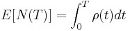
The prototypes produced during the development have design, manufacturing and/or engineering deficiencies whose correction, entails being subjected to a rigorous testing program to identify and appropriate corrective actions (or redesign). Reliability growth is the improvement in the reliability of a product (component, subsystem or system) over a period of time due to changes in the product’s design and/or the manufacturing process.
The concept of reliability growth is not just theoretical or absolute. Reliability growth is related to factors such as the management strategy toward taking corrective actions, effectiveness of the fixes, reliability requirements, the initial reliability level, reliability funding and competitive factors. For example, one management team may take corrective actions for 90% of the failures seen during testing, while another management team with the same design and test information may take corrective actions on only 65% of the failures seen during testing. Different management strategies may attain different reliability values with the same basic design. The effectiveness of the corrective actions is also relative when compared to the initial reliability at the beginning of testing. If corrective actions give a 400% improvement in reliability for equipment that initially had one tenth of the reliability goal, this is not as significant as a 50% improvement in reliability if the system initially had one half the reliability goal.
Elements of a Reliability Growth Program
In a formal reliability growth program a reliability goal (or goals) is set and should be achieved during the development testing program with the necessary allocation or reallocation of resources. Therefore, planning and evaluating are essential factors in a growth process program. A comprehensive reliability growth program needs well-structured planning of the assessment techniques. A reliability growth program differs from a conventional reliability program in that there is a more objectively developed growth standard against which assessment techniques are compared. A comparison between the assessment and the planned value provides a good estimate of whether or not the program is progressing as scheduled. If the program does not progress as planned, then new strategies should be considered. For example, a reexamination of the problem areas may result in changing the management strategy so that more problem failure modes surfaced during the testing actually receive a corrective action instead of a repair. Several important factors for an effective reliability growth program are:
- Management: the decisions are made regarding the management strategy to correct problems or not correct problems and the effectiveness of the corrective actions
- Testing: provides opportunities to identify the weaknesses and failure modes in the design and manufacturing process
- Failure mode root cause identification: funding, personnel and procedures are provided to analyze, isolate and identify the cause of failures
- Corrective action effectiveness: design resources to implement corrective actions that are effective and support attainment of the reliability goals
- Valid reliability assessments
Reliability growth studies are necessary to insure that, based on information available at the beginning of a project, the reliability, R, MTBF, m, or failure rate, λ, goals are capable of being met by acceptance or delivery and use time. This growth model is normally used to project R, m or λ at the completion date. If this projected R, m or λ is equal to or exceeds the specified target goal, then the project manager would be confident that the project’s R, m or λ requirements will be met. Otherwise, the manager will have to re-assess the reliability prediction techniques or refine them in the hopes of exceeding the goal.
During the early stages of developing and prototyping complex systems, reliability often does not meet customer requirements. A formal test procedure aimed at discovering and fixing causes of unreliability is known as a Reliability Improvement Test. This test focuses on system design, system assembly and component selection weaknesses that cause failures.
A typical reliability improvement test procedure would be to run a prototype system, as the customer might for a period of several weeks, while a multi-disciplined team of engineers and technicians (design, quality, reliability, manufacturing, etc.) analyze every failure that occurs. This team comes up with root causes for the failures and develops design and/or assembly improvements to hopefully eliminate or reduce the future occurrence of that type of failure. As the testing continues, the improvements the team comes up with are incorporated into the prototype, so it is expected that reliability will improve during the course of the test.
Another name for reliability improvement testing is TAAF testing, standing for Test, Analyze And Fix. While only one model applies when a repairable system has no improvement or degradation trends (the constant repair rate HPP model), there are infinitely many models that could be used to describe a system with a decreasing repair rate (reliability growth models).
Fortunately, one or two relatively simple models have been very successful in a wide range of industrial applications. Two models are the NHPP Power Law Model and the NHPP Exponential Law Model. The Power Law Model underlies the frequently used graphical technique known as Duane Plotting.
Reliability Growth Plots
Reliability growth plots have a variety of names known as: Duane plots, Crow plots, Crow AMSAA plots, Crow-AMSAA plots, Crow/AMSAA plots, C/A plots, and C-A plots. They are log-log plots showing reliability trends of improvement, deterioration, or no-change (no improvement or deterioration). The most common plot is cumulative failures versus cumulative time. Often the Y-axis is transformed to plot cumulative mean time versus cumulative time which makes it easy to interpret—when the line slope is upward and to the right, reliability is improving; likewise when it is trending downward and to the right, reliability is deteriorating.
The plots are “show me, don’t tell me” how failures are occurring with time. You can use your maintenance data records to forecast future failures. Also you can see the results of improvement programs and easily calculate the changes from the straight lines and the cusps produced by improvement programs.
Reliability growth plots showing how reliability changes over time with simple graphics plotted in a log-log format. Fortunately, the trend lines often have straight line segments, and this makes predictions of future failures a simple matter.
The Duane Method
It is common for new products to be less reliable during early development than later in the programme, when improvements have been incorporated as a result of failures observed and corrected. Similarly, products in service often display reliability growth. This was first analysed by J. T. Duane, who derived an empirical relationship based upon observation of the MTBF improvement of a range of items used on aircraft. Duane observed that the cumulative MTBF θc (total time divided by total failures) plotted against total time on log–log paper gave a straight line. The slope ( α ) gave an indication of reliability (MTBF) growth, that is
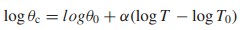
where θ0 is the cumulative MTBF at the start of the monitoring period T0. Therefore,
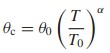
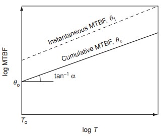
The relationship is shown plotted in figure below. The slope α gives an indication of the rate of MTBF growth and hence the effectiveness of the reliability programme in correcting failure modes. Duane observed that typically α ranged between 0.2 and 0.4, and that the value was correlated with the intensity of the effort on reliability improvement.
The Duane method is applicable to a population with a number of failure modes which are progressively corrected, and in which a number of items contribute different running times to the total time. Therefore it is not appropriate for monitoring early development testing, and it is common for early test results to show a poor fit to the Duane model.
We can derive the instantaneous MTBF θi of the population, as

The Duane plot is a scatterplot of the cumulative failure rate over time, and helps you assess whether your system is improving, deteriorating, or remaining stable over time.
The fitted line on the Duane plot is the best fitted line when the assumption of the power-law process is valid and the shape and scale are estimated using the least squares estimation method. The slope of the fitted line on a Duane plot is the estimated shape parameter minus 1. Use a Duane plot for these purposes
- To assess whether your data follow a power-law process or a homogeneous Poisson process. The Duane plot is usually approximately linear if the power-law process or homogeneous Poisson process is appropriate.
- To determine whether your system is improving, deteriorating, or remaining stable.
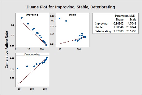
A negative slope shows reliability improvement. A positive slope shows reliability deterioration. No slope (a horizontal line) shows a stable system.
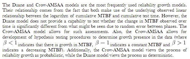
Crow-AMSAA Model
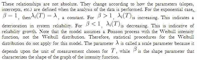
The Duane Model could be stochastically represented as a Weibull process, allowing for statistical procedures to be used in the application of this model in reliability growth. This statistical extension became what is known as the Crow-AMSAA (NHPP) model. This method was first developed at the U.S. Army Materiel Systems Analysis Activity (AMSAA). It is frequently used on systems when usage is measured on a continuous scale. It can also be applied for the analysis of one shot items when there is high reliability and a large number of trials.
Test programs are generally conducted on a phase by phase basis. The Crow-AMSAA model is designed for tracking the reliability within a test phase and not across test phases. A development testing program may consist of several separate test phases. If corrective actions are introduced during a particular test phase, then this type of testing and the associated data are appropriate for analysis by the Crow-AMSAA model. The model analyzes the reliability growth progress within each test phase and can aid in determining the following
- Reliability of the configuration currently on test
- Reliability of the configuration on test at the end of the test phase
- Expected reliability if the test time for the phase is extended
- Growth rate
- Confidence intervals
- Applicable goodness-of-fit tests
The reliability growth pattern for the Crow-AMSAA model is exactly the same pattern as for the Duane postulate, that is, the cumulative number of failures is linear when plotted on ln-ln scale. Unlike the Duane postulate, the Crow-AMSAA model is statistically based. Under the Duane postulate, the failure rate is linear on ln-ln scale. However, for the Crow-AMSAA model statistical structure, the failure intensity of the underlying non-homogeneous Poisson process (NHPP) is linear when plotted on ln-ln scale.
Let ![]() be the cumulative number of failures observed in cumulative test time
be the cumulative number of failures observed in cumulative test time ![]() , and let
, and let ![]() be the failure intensity for the Crow-AMSAA model. Under the NHPP model,
be the failure intensity for the Crow-AMSAA model. Under the NHPP model, ![]() is approximately the probably of a failure occurring over the interval
is approximately the probably of a failure occurring over the interval ![]() for small
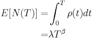
for small ![]() In addition, the expected number of failures experienced over the test interval
In addition, the expected number of failures experienced over the test interval ![]() under the Crow-AMSAA model is given by:
under the Crow-AMSAA model is given by:
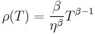
The Crow-AMSAA model assumes that ![]() may be approximated by the Weibull failure rate function:
may be approximated by the Weibull failure rate function:

Therefore, if ![]() the intensity function,
the intensity function, ![]() or the instantaneous failure intensity,
or the instantaneous failure intensity, ![]() , is defined as:
, is defined as:
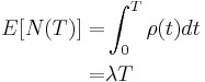
In the special case of exponential failure times, there is no growth and the failure intensity, ![]() is equal to
is equal to ![]() . In this case, the expected number of failures is given by:
. In this case, the expected number of failures is given by:
In order for the plot to be linear when plotted on ln-ln scale under the general reliability growth case, the following must hold true where the expected number of failures is equal to:
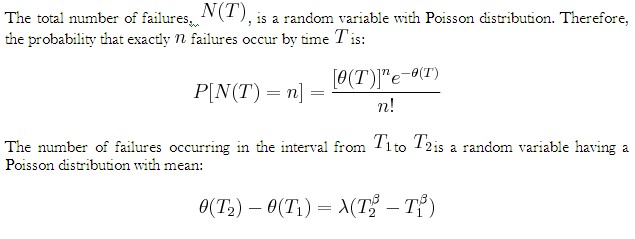
To put a statistical structure on the reliability growth process, consider again the special case of no growth. In this case the number of failures, ![]() experienced during the testing over
experienced during the testing over ![]() is random. The expected number of failures,
is random. The expected number of failures, ![]() is said to follow the homogeneous (constant) Poisson process with mean
is said to follow the homogeneous (constant) Poisson process with mean ![]() and is given by:
and is given by:
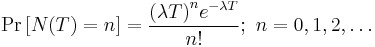
The Crow-AMSAA model generalizes this no growth case to allow for reliability growth due to corrective actions. This generalization keeps the Poisson distribution for the number of failures but allows for the expected number of failures,![]() to be linear when plotted on ln-ln scale.
to be linear when plotted on ln-ln scale.
The Crow-AMSAA model lets ![]() . The probability that the number of failures,
. The probability that the number of failures,![]() will be equal to π under growth is then given by the Poisson distribution.
will be equal to π under growth is then given by the Poisson distribution.

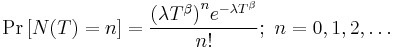
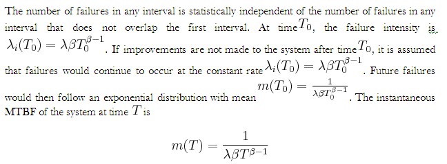
This is the general growth situation, and the number of failures, ![]() follows a non-homogeneous Poisson process. The exponential, “no growth” homogeneous Poisson process is a special case of the non-homogeneous Crow-AMSAA model. This is reflected in the Crow-AMSAA model parameter where
follows a non-homogeneous Poisson process. The exponential, “no growth” homogeneous Poisson process is a special case of the non-homogeneous Crow-AMSAA model. This is reflected in the Crow-AMSAA model parameter where ![]() . The cumulative failure rate,
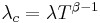
. The cumulative failure rate, ![]() is
is
The cumulative ![]() is:
is:
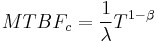
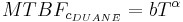
As mentioned above, the local pattern for reliability growth within a test phase is the same as the growth pattern observed by Duane. The Duane ![]() is equal to:
is equal to:
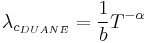
And the Duane cumulative failure rate, ![]() , is:
, is:
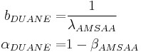
Thus a relationship between Crow-AMSAA parameters and Duane parameters can be developed, such that:


![]() is also called the demonstrated (or achieved) MTBF.
is also called the demonstrated (or achieved) MTBF.