Probability Distribution

Probability is a measure of the likeliness that an event will occur. Probability is used to quantify an attitude of mind towards some proposition of whose truth we are not certain.

Concepts

Basic probability concepts and terminology is discussed below

• Probability – It is the chance that something will occur. It is expressed as a decimal fraction or a percentage. It is the ratio of the chances favoring an event to the total number of chances for and against the event. The probability of getting 4 with a rolling of dice, is 1 (count of 4 in a dice) / 6 = .01667. Probability then can be the number of successes divided by the total number of possible occurrences. Pr(A) is the probability of event A. The probability of any event (E) varies between 0 (no probability) and 1 (perfect probability).
• Sample Space – It is the set of possible outcomes of an experiment or the set of conditions. The sample space is often denoted by the capital letter S. Sample space outcomes are denoted using lower-case letters (a, b, c . . .) or the actual values like for a dice, S={1,2,3,4,5,6}
• Event – An event is a subset of a sample space. It is denoted by a capital letter such as A, B, C, etc. Events have outcomes, which are denoted by lower-case letters (a, b, c . . .) or the actual values if given like in rolling of dice, S={1,2,3,4,5,6}, then for event A if rolled dice shows 5 so, A ={5}. The sum of the probabilities of all possible events (multiple E’s) in total sample space (S) is equal to 1.
• Independent Events – Each event is not affected by any other events for example tossing a coin three times and it comes up “Heads” each time, the chance that the next toss will also be a “Head” is still 1/2 as every toss is independent of earlier one.
• Dependent Events – They are the events which are affected by previous events like drawing 2 Cards from a deck will reduce the population for second card and hence, it’s probability as after taking one card from the deck there are less cards available as the probability of getting a King, for the 1st time is 4 out of 52 but for the 2nd time is 3 out of 51.
• Simple Events – An event that cannot be decomposed is a simple event (E). The set of all sample points for an experiment is called the sample space (S).
• Compound Events – Compound events are formed by a composition of two or more events. The two most important probability theorems are the additive and multiplicative laws.
• Union of events – The union of two events is that event consisting of all outcomes contained in either of the two events. The union is denoted by the symbol U placed between the letters indicating the two events like for event A={1,2} and event B={2,3} i.e. outcome of event A can be either 1 or 2 and of event B is 2 or 3 then, AUB = {1,2}
• Intersection of events – The intersection of two events is that event consisting of all outcomes that the two events have in common. The intersection of two events can also be referred to as the joint occurrence of events. The intersection is denoted by the symbol ∩ placed between the letters indicating the two events like for event A={1,2} and event B={2,3} then, A∩B = {2}
• Complement – The complement of an event is the set of outcomes in the sample space that are not in the event itself. The complement is shown by the symbol ` placed after the letter indicating the event like for event A={1,2} and Sample space S={1,2,3,4,5,6} then A`={3,4,5,6}
• Mutually Exclusive – Mutually exclusive events have no outcomes in common like the intersection of an event and its complement contains no outcomes or it is an empty set, Ø for example if A={1,2} and B={3,4} and A ∩ B= Ø.
• Equally Likely Outcomes – When a sample space consists of N possible outcomes, all equally likely to occur, then the probability of each outcome is 1/N like the sample space of all the possible outcomes in rolling a die is S = {1, 2, 3, 4, 5, 6}, all equally likely, each outcome has a probability of 1/6 of occurring but, the probability of getting a 3, 4, or 6 is 3/6 = 0.5.
• Probabilities for Independent Events or multiplication rule – Independent events occurrence does not depend on other events of sample space then the probability of two events A and B occurring both is P(A ∩ B) = P(A) x P(B) and similarly for many events the independence rule is extended as P(A∩B∩C∩. . .) = P(A) x P(B) x P(C) . . . This rule is also called as the multiplication rule. For example the probability of getting three times 6 in rolling a dice is 1/6 x 1/6 x 1/6 = 0.00463
• Probabilities for Mutually Exclusive Events or Addition Rule – Mutually exclusive events do not occur at the same time or in the same sample space and do not have any outcomes in common. Thus, for two mutually exclusive events, A and B, the event A∩B = Ø, and the probability of events A and B occurring is zero, as P(A∩B) = 0, for events A and B, the probabilities of either or both of the events occurring is P(AUB) = P(A) + P(B) – P(A∩B) also called as addition rule.For example let P(A) = 0.2, P(B) = 0.4, and P(A∩B) = 0.5, then P(AUB) = P(A) + P(B) – P(A∩B) = 0.2 + 0.4 – 0.5 = 0.1

Conditional Probability

It is the result of an event depending on the sample space or another event. The conditional probability of an event (the probability of event A occurring given that event B has already occurred) can be found as

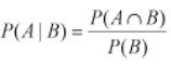
It can also be referred as –

P(B|A) = P(A and B) / P(A)

Since we are given that event A has occurred, we have a reduced sample space. Instead of the entire sample space S, we now have a sample space of A since we know A has occurred. So the old rule about being the number in the event divided by the number in the sample space still applies. It is the number in A and B (must be in A since A has occurred) divided by the number in A. If you then divided numerator and denominator of the right hand side by the number in the sample space S, then you have the probability of A and B divided by the probability of A.

For example in sample set of 100 items received from supplier1 (total supplied= 60 items and reject items = 4) and supplier 2(40 items), event A is the rejected item and B be the event if item from supplier1. Then, probability of reject item from supplier1 is – P(A|B) = P(A∩B)/ P(B), P(A∩B) = 4/100 and P(B) = 60/100 = 1/15.

You toss two pennies. The first penny shows HEADS and the other penny rolls under the table and you cannot see it. Now, what is the probability that they are both HEADS? Since you already know that one is HEADS, the probability of getting HEADS on the second penny is 1 out of 2.

The probability changes if you have partial information. This “affected” probability is called conditional probability. Notation for conditional probability: P(B|A), is read as, the probability of B given A.

Bayes’ Theorem

Bayes’ Theorem is a theorem of probability theory originally stated by the Reverend Thomas Bayes. It can be seen as a way of understanding how the probability that a theory is true is affected by a new piece of evidence. It has been used in a wide variety of contexts, ranging from marine biology to the development of “Bayesian” spam blockers for email systems. In the philosophy of science, it has been used to try to clarify the relationship between theory and evidence. Many insights in the philosophy of science involving confirmation, falsification, the relation between science and pseudosience, and other topics can be made more precise, and sometimes extended or corrected, by using Bayes’ Theorem.

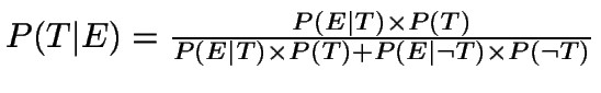
In this formula, T stands for a theory or hypothesis that we are interested in testing, and E represents a new piece of evidence that seems to confirm or disconfirm the theory. For any proposition S, we will use P(S) to stand for our degree of belief, or “subjective probability,” that S is true. In particular, P(T) represents our best estimate of the probability of the theory we are considering, prior to consideration of the new piece of evidence. It is known as the prior probability of T.

What we want to discover is the probability that T is true supposing that our new piece of evidence is true. This is a conditional probability, the probability that one proposition is true provided that another proposition is true. For instance, suppose you draw a card from a deck of 52, without showing it to me. Assuming the deck has been well shuffled, I should believe that the probability that the card is a jack, P(J), is 4/52, or 1/13, since there are four jacks in the deck. But now suppose you tell me that the card is a face card. The probability that the card is a jack, given that it is a face card, is 4/12, or 1/3, since there are 12 face cards in the deck. We represent this conditional probability as P(J|F), meaning the probability that the card is a jack given that it is a face card.

(We don’t need to take conditional probability as a primitive notion; we can define it in terms of absolute probabilities: P(A|B) = P(A and B) / P(B), that is, the probability that A and B are both true divided by the probability that B is true.)

Using this idea of conditional probability to express what we want to use Bayes’ Theorem to discover, we say that P(T|E), the probability that T is true given that E is true, is the posterior probability of T. The idea is that P(T|E) represents the probability assigned to T after taking into account the new piece of evidence, E. To calculate this we need, in addition to the prior probability P(T), two further conditional probabilities indicating how probable our piece of evidence is depending on whether our theory is or is not true. We can represent these as P(E|T) and P(E|~T), where ~T is the negation of T, i.e. the proposition that T is false.

Contingency Table

A contingency table (also referred to as cross tabulation or crosstab) is a type of table in a matrix format that displays the (multivariate) frequency distribution of the variables. They are heavily used in survey research, business intelligence, engineering and scientific research. They provide a basic picture of the interrelation between two variables and can help find interactions between them. The term contingency table was first used by Karl Pearson in “On the Theory of Contingency and Its Relation to Association and Normal Correlation”, part of the Drapers’ Company Research Memoirs Biometric Series I published in 1904.

A crucial problem of multivariate statistics is finding (direct-)dependence structure underlying the variables contained in high-dimensional contingency tables. If some of the conditional independences are revealed, then even the storage of the data can be done in a smarter way (see Lauritzen (2002)). In order to do this one can use information theory concepts, which gain the information only from the distribution of probability, which can be expressed easily from the contingency table by the relative frequencies.

Example – Suppose that we have two variables, sex (male or female) and handedness (right- or left-handed). Further suppose that 100 individuals are randomly sampled from a very large population as part of a study of sex differences in handedness. A contingency table can be created to display the numbers of individuals who are male and right-handed, male and left-handed, female and right-handed, and female and left-handed. Such a contingency table is shown below.

	Right-handed	Left-handed	Total
Males	43	9	52
Females	44	4	48
Totals	87	13	100

The numbers of the males, females, and right- and left-handed individuals are called marginal totals. The grand total, i.e., the total number of individuals represented in the contingency table, is the number in the bottom right corner.

The table allows us to see at a glance that the proportion of men who are right-handed is about the same as the proportion of women who are right-handed although the proportions are not identical. The significance of the difference between the two proportions can be assessed with a variety of statistical tests including Pearson’s chi-squared test, the G-test, Fisher’s exact test, and Barnard’s test, provided the entries in the table represent individuals randomly sampled from the population about which we want to draw a conclusion. If the proportions of individuals in the different columns vary significantly between rows (or vice versa), we say that there is a contingency between the two variables. In other words, the two variables are not independent. If there is no contingency, we say that the two variables are independent.

The example above is the simplest kind of contingency table, a table in which each variable has only two levels; this is called a 2 × 2 contingency table. In principle, any number of rows and columns may be used. There may also be more than two variables, but higher order contingency tables are difficult to represent on paper. The relation between ordinal variables, or between ordinal and categorical variables, may also be represented in contingency tables, although such a practice is rare.

Standard contents of a contingency table

• Multiple columns (historically, they were designed to use up all the white space of a printed page). Where each column refers to a specific sub-group in the population (e.g., men), the columns are sometimes referred to as banner points or cuts (and the rows are sometimes referred to as stubs).
• Significance tests. Typically, either column comparisons, which test for differences between columns and display these results using letters, or, cell comparisons, which use color or arrows to identify a cell in a table that stands out in some way (as in the example above).
• Nets or netts which are sub-totals.
• One or more of: percentages, row percentages, column percentages, indexes or averages.
• Unweighted sample sizes (i.e., counts).

Permutation and Combination

Permutations are for lists (order matters) and combinations are for groups (order doesn’t matter).

Permutation

It relates to the act of rearranging, or permuting, all the members of a set into some sequence or order (unlike combinations, which are selections of some members of the set where order is disregarded). For example, written as tuples, there are six permutations of the set {1,2,3}, namely: (1,2,3), (1,3,2), (2,1,3), (2,3,1), (3,1,2), and (3,2,1). As another example, an anagram of a word, all of whose letters are different, is a permutation of its letters.

The number of permutations of n distinct objects is n factorial usually written as n!, which means the product of all positive integers less than or equal to n.

In algebra and particularly in group theory, a permutation of a set S is defined as a bijection from S to itself. That is, it is a function from S to S for which every element occurs exactly once as an image value. This is related to the rearrangement of the elements of S in which each element s is replaced by the corresponding f(s). The collection of such permutations form a group called the symmetric group of S. The key to this group’s structure is the fact that the composition of two permutations (performing two given rearrangements in succession) results in another rearrangement. Permutations may act on structured objects by rearranging their components, or by certain replacements (substitutions) of symbols.

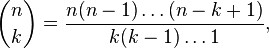
The number of ways of obtaining an ordered subset of elements from a set of elements is given by 

where is a factorial. For example, there are  2-subsets of , namely , , , , , , , , , , , and . The unordered subsets containing  elements are known as the k-subsets of a given set.

Combination

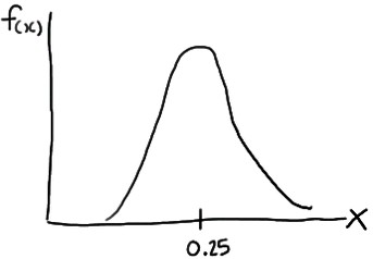
It is a way of selecting items from a collection, such that (unlike permutations) the order of selection does not matter. In smaller cases it is possible to count the number of combinations. For example given three fruits, say an apple, an orange and a pear, there are three combinations of two that can be drawn from this set: an apple and a pear; an apple and an orange; or a pear and an orange. More formally, a k-combination of a set S is a subset of k distinct elements of S. If the set has n elements, the number of k-combinations is equal to the binomial coefficient

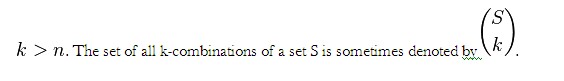
Combinations refer to the combination of n things taken k at a time without repetition. To refer to combinations in which repetition is allowed, the terms k-selection, k-multiset, or k-combination with repetition are often used. If, in the above example, it was possible to have two of any one kind of fruit there would be 3 more 2-selections: one with two apples, one with two oranges, and one with two pears.

 where is a factorial. For example, there arecombinations of two elements out of the set {1,2,3,4}, namely {1,2}, {1,3}, {1,4}, {2,3}, {2,4} and {3,4}. These combinations are known as k-subsets.

Rules of Probability

Rule 1: The probability of an impossible event is zero; the probability of a certain event is one. Therefore, for any event A, the range of possible probabilities is: 0 ≤ P(A) ≤ 1

Rule 2: For S the sample space of all possibilities, P(S) = 1. That is the sum of all the probabilities for all possible events is equal to one. Recall the party affiliation above: if you have to belong to one of the three designated political parties, then the sum of P(R), P(D) and P(I) is equal to one.

Rule 3 or Rule of Subtraction The probability that event A will occur is equal to 1 minus the probability that event A will not occur. P(A) = 1 – P(A’) For any event A, P(A^c) = 1 – P(A). It follows then that P(A) = 1 – P(A^c)

Rule 4 (Addition Rule): This is the probability that either one or both events occur

1. If two events, say A and B, are mutually exclusive – that is A and B have no outcomes in common – then P(A or B) = P(A) + P(B)
2. If two events are NOT mutually exclusive, then P(A or B) = P(A) + P(B) – P(A and B)

The probability that Event A or Event B occurs is equal to the probability that Event A occurs plus the probability that Event B occurs minus the probability that both Events A and B occur, as

P(A ∪ B) = P(A) + P(B) – P(A ∩ B))

Invoking the fact that P(A ∩ B) = P( A )P( B | A ), the Addition Rule can also be expressed as

P(A ∪ B) = P(A) + P(B) – P(A)P( B | A )

Rule 5 (Multiplication Rule): This is the probability that both events occur

1. P(A and B) = P(A) × P(B|A) or P(B) × P(A|B) Note: this straight line symbol, ‘ | ‘, does not mean divide! This symbols means “conditional” or “given”. For instance P(A|B) means the probability that event A occurs given event B has occurred.
2. If A and B are independent – neither event influences or affects the probability that the other event occurs – then P(A and B) = P(A) × P(B) . This particular rule extends to more than two independent events. For example, P(A and B and C) = P(A) × P(B) × P(C)

Rule 6 (Conditional Probability): P(A|B)=P(A and B)P(B) or P(B|A)=P(A and B)P(A)

Probabilistic Distributions

Distribution – Prediction and decision-making needs fitting data to distributions (like normal, binomial, or Poisson). A probability distribution identifies whether a value will occur within a given range or the probability that a value that is lesser or greater than x will occur or the probability that a value between x and y will occur.

A distribution is the amount of variation in the outputs of a process, expressed by shape (symmetry, skewness and kurtosis), average and standard deviation. Symmetrical distributions the mean represents the central tendency of the data but for skewed distributions, the median is the indicator. The standard deviation provides a measure of variation from the mean. Similarly skewness is a measure of the location of the mode relative to the mean thus, if mode is to the mean’s left then the skewness is negative else positive but for symmetrical distribution, skewness is zero. Kurtosis measures the peakness or relative flatness of the distribution and the kurtosis is higher for a higher and narrower peak.

Probability Distribution – It is a mathematical formula relating the values of a characteristic or attribute with their probability of occurrence in the population. It depicts the possible events and the associated probability for each of these events to occur. Probability distribution is divided as

• Discrete data describe a finite set of possible occurrences for the data like rolling a dice with the random variable can take value from 1, 2, 3, 4, 5 or 6. The most used discrete probability distributions are the binomial, the Poisson, the geometric, and the hypergeometric distribution.
• Continuous data describes a continuum of possible occurrences that is unbroken as, the distribution of body weight is a random variable with infinite number of possible data points.

Probability Density Function – Probability distributions for continuous variables use probability density functions (or PDF), which are mathematically model the probability density shown in a histogram but, discrete variables have probability mass function. PDFs employ integrals as the summation of area between two points when used in a equation. If a histogram shows the relative frequencies of a series of output ranges of a random variable, then the histogram also depicts the shape of the probability density for the random variable hence, the shape of the probability density function is also described as the shape of the distribution. An example illustrates it

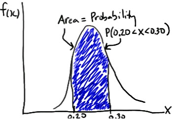
Example: A fast-food chain advertises a burger weighing a quarter-kg but, it is not exactly 0.25 kg. One randomly selected burger might weigh 0.23 kg or 0.27 kg. What is the probability that a randomly selected burger weighs between 0.20 and 0.30 kg? That is, if we let X denote the weight of a randomly selected quarter-kg burger in kg, what is P(0.20 < X < 0.30)?

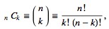
This problem is solved by using probability density function as, imagine randomly selecting, 100 burgers advertised to weigh a quarter-kg. If weighed the 100 burgers, and created a density histogram of the resulting weights, perhaps the histogram might be

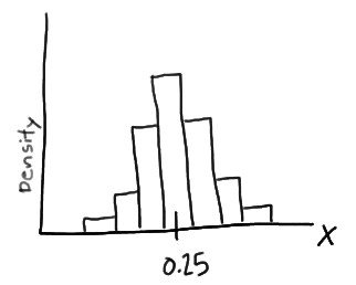
In this case, the histogram illustrates that most of the sampled burgers do indeed weigh close to 0.25 kg, but some are a bit more and some a bit less. Now, what if we decreased the length of the class interval on that density histogram then, it will be as

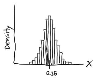
Now, if it is pushed further and the interval is decreased then, the intervals would eventually get small that we could represent the probability distribution of X, not as a density histogram, but rather as a curve (by connecting the “dots” at the tops of the tiny rectangles) as

Such a curve is denoted f(x) and is called a (continuous) probability density function. A density histogram is defined so that the area of each rectangle equals the relative frequency of the corresponding class, and the area of the entire histogram equals 1. Thus, finding the probability that a continuous random variable X falls in some interval of values involves finding the area under the curve f(x) sandwiched by the endpoints of the interval. In the case of this example, the probability that a randomly selected burger weighs between 0.20 and 0.30 kg is then this area, as

Distributions Types – Various distributions are

• Binomial – It is used in finite sampling problems when each observation has only one of two possible outcomes, such as pass/fail.
• Poisson – It is used for situations when an attribute possibility is that each sample can have multiple defects or failures.
• Normal – It is characterized by the traditional “bell-shaped” curve, the normal distribution is applied to many situations with continuous data that is roughly symmetrical around the mean.
• Chi-square – It is used in many situations when an inference is drawn on a single variance or when testing for goodness of fit or independence. Examples of use of this distribution include determining the confidence interval for the standard deviation of a population or comparing the frequency of variables.
• Student’s t – It is used in many situations when inferences are drawn without a variance known in the case of a single mean or the comparison of two means.
• F – It is used in situations when inferences are drawn from two variances such as whether two population variances are different in magnitude.
• Hypergeometric – It is the “true” distribution. It is used in a similar manner to the binomial distribution except that the sample size is larger relative to the population. This distribution should be considered whenever the sample size is larger than 10% of the population. The hypergeometric distribution is the appropriate probability model for selecting a random sample of n items from a population without replacement and is useful in the design of acceptance-sampling plans.
• Bivariate – It is created with the joint frequency distributions of modeled variables.
• Exponential – It is used for instances of examining the time between failures.
• Lognormal – It is used when raw data is skewed and the log of the data follows a normal distribution. This distribution is often used for understanding failure rates or repair times.
• Weibull – It is used when modeling failure rates particularly when the response of interest is percent of failures as a function of usage (time).

Binomial Distribution – It is used to model discrete data having only two possible outcomes like pass or fail, yes or no and which are exactly two mutually exclusive outcomes. It may be used to find the proportion of defective units produced by a process and used when population is large – when N> 50 with small size of sample compared to the population. The ideal situation is when sample size (n) is less than 10% of the population (N) or n< 0.1N. The binomial distribution is useful to find the number of defective products if the product either passes or fails a given test. The mean, variance, and standard deviation for a binomial distribution are µ = np, σ2= npq and σ =√npq. The essential conditions for a random variable are fixed number of observations (n) which are independent of each other, every trial results in either of the two possible outcomes and if the probability of a success is p and the probability of a failure is 1 -p.

The binomial probability distribution equation will show the probability p (the probability of defective) of getting x defectives (number of defectives or occurrences) in a sample of n units (or sample size) as

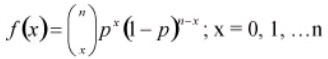
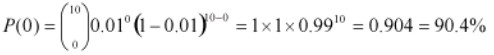
As an example if a product with a 1% defect rate, is tested with ten sample units from the process, Thus, n= 10, x= 0 and p= .01 then, the probability that there will be 0 defective products is

Poisson Distribution – It estimates the number of instances a condition of interest occurs in a process or population. It focuses on the probability for a number of events occurring over some interval or continuum where µ, the average of such an event occurring, is known like project team may want to know the probability of finding a defective part on a manufactured circuit board. Most frequently, this distribution is used when the condition may occur multiple times in one sample unit and user is interested in knowing the number of individual characteristics found like critical attribute of a manufactured part is measured in a random sampling of the production process with non-conforming conditions being recorded for each sample. The collective number of failures from the sampling may be modeled using the Poisson distribution. It can also be used to project the number of accidents for the following year and their probable locations. The essential condition for a random variable to follow Poisson distribution is that counts are independent of each other and the probability that a count occurs in an interval is the same for all intervals. The mean and the variance of the Poisson distribution are the same, and the standard deviation is the square root of the mean hence, µ = σ2 and σ =√µ =√σ2.

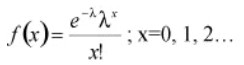
The Poisson distribution can be an approximation to the binomial when p is equal to or less than 0.1, and the sample size n is fairly large (generally, n >= 16) by using np as the mean of the Poisson distribution. Considering f(x) as the probability of x occurrences in the sample/interval, λ as the mean number of counts in an interval (where λ > 0), x as the number of defects/counts in the sample/interval and e as a constant approximately equal to 2.71828 then the equation for the Poisson distribution is as

Normal Distribution – A distribution is said to be normal when most of the observations are clustered around the mean. It charts a data set of which most of the data points are concentrated around the average (mean) in a symmetrical manner, thus forming a bell-shaped curve. The normal distribution’s shape is unique in that the most frequently occurring value is in the middle of the range and other probabilities tail off symmetrically in both directions. The normal distribution is used for continuous (measurement) data that is symmetric about the mean. The graph of the normal distribution depends on the mean and the variance. When the variance is large, the curve is short and wide and when the variance is small, the curve is tall and narrow.

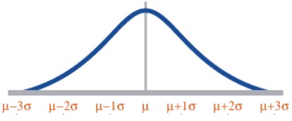
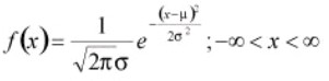
The normal distribution is also called as the Gaussian or standard bell distribution. The population mean μ is zero and that the population variance σ2 equals one as in the figure and σ is the standard deviation. The normal probability density function is

For normal distribution, the area under the curve lies between µ − σ and µ + σ.

Z- transformation – The shape of the normal distribution depends on two factors, the mean and the standard deviation. Every combination of µ and σ represent a unique shape of a normal distribution. Based on the mean and the standard deviation, the complexity involved in the normal distribution can be simplified and it can be converted into the simpler z-distribution. This process leads to the standardized normal distribution, Z = (X − µ)/σ. Because of the complexity of the normal distribution, the standardized normal distribution is often used instead.

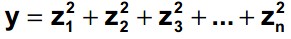
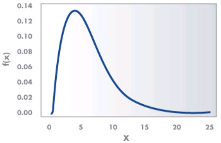
Chi-Square Distribution – The chi-square (χ2) distribution is used when testing a population variance against a known or assumed value of the population variance. It is skewed to the right or with a long tail toward the large values of the distribution. The overall shape of the distribution will depend on the number of degrees of freedom in a given problem. The degrees of freedom are 1 less than the sample size. It is formed by adding the squares of standard normal random variables. For example, if z is a standard normal random variable, then the following is a chi-square random variable (statistic) with n degrees of freedom.

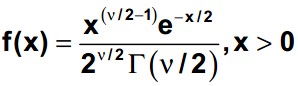
The chi-square probability density function where v is the degree of freedom and (x) is the gamma function is

An example of a χ2 distribution with 6 degrees of freedom is as

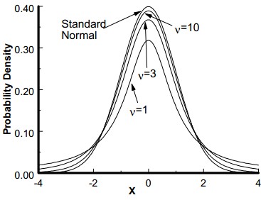
Student t Distribution – It was developed by W.S. Gosset. The t distribution is used to determine the confidence interval of the population mean and confidence statistics when comparing the means of sample populations but, the degrees of freedom for the problem must be know n. The degrees of freedom are 1 less than the sample size.

The student’s t distribution is a symmetrical continuous distribution and similar to the normal distribution, but the extreme tail probabilities are larger than for the normal distribution for sample sizes of less than 31. The shape and area of the t distribution approaches towards the normal distribution as the sample size increases. The t distribution can be used whenever samples are drawn from populations possessing a normal, bell-shaped distribution. There is a family of curves, one for each sample size from n =2 to n = 31.

F Distribution – The F distribution or F-test is a tool used for assessing the ratio of independent variances or equality of variances from two normal populations. It is used in the Analysis of Variance (ANOVA, a technique frequently used in the Design of Experiments to test for significant differences in variance within and between test runs).

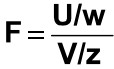
If U and V are the variances of independent random samples of size n and m taken from normally distributed populations with variances of w and z, then

which is a random variable with an F distribution with v1 = n-1 and v2 = m – 1. The F-distribution is represented by

with (s1)2 is the variance of the first sample (n1- 1 degrees of freedom in the numerator) and (s2)2 is the variance of the second sample (n2- 1 degrees of freedom in the denominator), given two random samples drawn from a normal distribution.

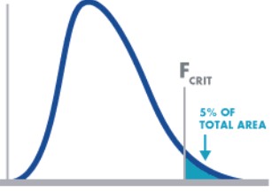
The shape of the F distribution is non-symmetrical and will depend on the number of degrees of freedom associated with (s1)2 and (s2)2. The distribution for the ratio of sample variances is skewed to the right (the large values).

Geometric Distribution – It addresses the number of trials necessary before the first success. If the trials are repeated k times until the first success, we would have k−1 failures. If p is the probability for a success and q the probability for a failure, the probability of the first success to occur at the kth trial is P(k, p) = p(q)k−1 with the mean and standard deviation are µ =1/p and σ = √q/p.

Hypergeometric Distribution – The hypergeometric distribution applies when the sample (n) is a relatively large proportion of the population (n >0.1N). The hypergeometric distribution is used when items are drawn from a population without replacement. That is, the items are not returned to the population before the next item is drawn out. The items must fall into one of two categories, such as good/bad or conforming/nonconforming.

The hypergeometric distribution is similar in nature to the binomial distribution, except the sample size is large compared to the population. The hypergeometric distribution determines the probability of exactly x number of defects when n items are samples from a population of N items containing D defects. The equation is

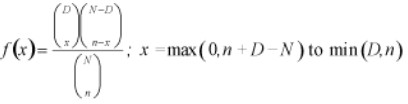
With, x is the number of nonconforming units in the sample (r is sometimes used here if dealing with occurrences), D is the number of nonconforming units in the population, N is the finite population size and n is the sample size.

Bivariate Distribution – When two variables are distributed jointly the resulting distribution is a bivariate distribution. Bivariate distributions may be used with either discrete or continuous data. The variables may be completely independent or a covariance may exist between them.

The bivariate normal distribution is a commonly used version of the bivariate distribution which may be used when there are two random variables. This equation was developed by Freund in 1962 as

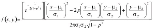
With

• -∞ < x < ∞
• -∞ < y < ∞
• -∞ < μ1< ∞
• -∞ < μ2< ∞
• σx> 0, σx> 0
• μ1 and μ2 are the two population means
• First σ2 and second σ2 are the two variances
• ρ is the correlation coefficient of the random variables

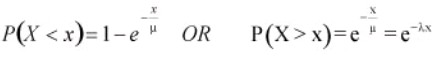
Exponential Distribution – It is used to analyze reliability, and to model items with a constant failure rate. The exponential distribution is related to the Poisson distribution and used to determine the average time between failures or average time between a numbers of occurrences. The mean and the standard deviation are µ =1/λ and σ =1/λ.

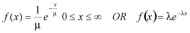
For example, if there is an average of 0.50 failures per hour (discrete data – Poisson distribution), then the mean time between failure (MTBF) is 1 / 0.50 = 2 hours (continuous data – exponential distribution). If a random variable x is distributed exponentially, then its reciprocal y =1/x follows a Poisson distribution. The opposite is also true. If x follows a Poisson distribution, then the reciprocal y = 1/x is exponentially distributed. The exponential distribution equation is

With μ is the mean (also sometimes referred to as θ), λ is the failure rate which is the same as1/μ and x is the x-axis values. When this equation is integrated, it results in cumulative probabilities as

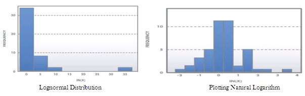
Lognormal Distribution – The most common transformation is made by taking the natural logarithm, but any base logarithm, such as base 10 or base 2 may be used. It is used to model various situations such as response time, time-to-failure data, and time-to-repair data. Lognormal distribution is a skewed-right distribution (with most data in the left tail), and consists of the distribution of the random variable whose logarithm follows the normal distribution.

The lognormal distribution assumes only positive values. When the data follows a lognormal distribution, a transformation of data can be done to make the data follow a normal distribution. Then probabilities, confidence intervals and tests of hypothesis can be conducted (if the data follows a normal distribution). The lognormal probability density function is

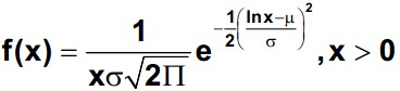
With μ is the location parameter or log mean and σ is the scale (or shape) parameter or standard deviation of natural logarithms of the individual values.

Weibull Distribution – The Weibull distribution is a widely used distribution for understanding reliability and is similar in appearance to the lognormal. It can be used to measure time to fail, time to repair, and material strength. The shape and dispersion of the Weibull distribution depends on two parameters β which is the shape parameter and θ which is the scale parameter but, both parameters are greater than zero.

The Weibull distribution is one of the most widely used distributions in reliability and statistical applications. The two and three parameter Weibull common versions. The difference is the three parameter Weibull distribution has a location parameter when there is some non-zero time to first failure. In general, the probabilities from a Weibull distribution can be found from the cumulative Weibull function as

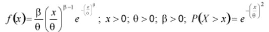
With, X is a random variable, x is an actual observation. The shape parameter (β) provides the Weibull distribution with its flexibility as

• If β = 1, the Weibull distribution is identical to the exponential distribution.
• If β = 2, the Weibull distribution is identical to the Rayleigh distribution.

If 3 < β < 4, then the Weibull distribution approximates a normal distribution.