Statistical inference is the process of deducing properties of an underlying distribution by analysis of data. Inferential statistical analysis infers properties about a population: this includes testing hypotheses and deriving estimates. The population is assumed to be larger than the observed data set; in other words, the observed data is assumed to be sampled from a larger population.
Inferential statistics can be contrasted with descriptive statistics. Descriptive statistics is solely concerned with properties of the observed data, and does not assume that the data came from a larger population.
Statistical inference makes propositions about a population, using data drawn from the population via some form of sampling. Given a hypothesis about a population, for which we wish to draw inferences, statistical inference consists of (firstly) selecting a statistical model of the process that generates the data and (secondly) deducing propositions from the model.
Konishi & Kitagawa state, “The majority of the problems in statistical inference can be considered to be problems related to statistical modeling”. Relatedly, Sir David Cox has said, “How [the] translation from subject-matter problem to statistical model is done is often the most critical part of an analysis”.
The conclusion of a statistical inference is a statistical proposition. Some common forms of statistical proposition are the following:
- a point estimate, i.e. a particular value that best approximates some parameter of interest;
- an interval estimate, e.g. a confidence interval (or set estimate), i.e. an interval constructed using a dataset drawn from a population so that, under repeated sampling of such datasets, such intervals would contain the true parameter value with the probability at the stated confidence level;
- a credible interval, i.e. a set of values containing, for example, 95% of posterior belief;
- rejection of a hypothesis;
- clustering or classification of data points into groups.
Estimation
One of the major applications of statistics is estimating population parameters from sample statistics. For example, a poll may seek to estimate the proportion of adult residents of a city that support a proposition to build a new sports stadium. Out of a random sample of 200 people, 106 say they support the proposition. Thus in the sample, 0.53 of the people supported the proposition. This value of 0.53 is called a point estimate of the population proportion. It is called a point estimate because the estimate consists of a single value or point.
Point estimates are usually supplemented by interval estimates called confidence intervals. Confidence intervals are intervals constructed using a method that contains the population parameter a specified proportion of the time. For example, if the pollster used a method that contains the parameter 95% of the time it is used, he or she would arrive at the following 95% confidence interval: 0.46 < π < 0.60. The pollster would then conclude that somewhere between 0.46 and 0.60 of the population supports the proposal. The media usually reports this type of result by saying that 53% favor the proposition with a margin of error of 7%.
In an experiment on memory for chess positions, the mean recall for tournament players was 63.8 and the mean for non-players was 33.1. Therefore a point estimate of the difference between population means is 30.7. The 95% confidence interval on the difference between means extends from 19.05 to 42.35.
Degrees of Freedom
Some estimates are based on more information than others. For example, an estimate of the variance based on a sample size of 100 is based on more information than an estimate of the variance based on a sample size of 5. The degrees of freedom (df) of an estimate is the number of independent pieces of information on which the estimate is based.
As an example, let’s say that we know that the mean height of Martians is 6 and wish to estimate the variance of their heights. We randomly sample one Martian and find that its height is 8. Recall that the variance is defined as the mean squared deviation of the values from their population mean. We can compute the squared deviation of our value of 8 from the population mean of 6 to find a single squared deviation from the mean. This single squared deviation from the mean, (8-6)2 = 4, is an estimate of the mean squared deviation for all Martians. Therefore, based on this sample of one, we would estimate that the population variance is 4. This estimate is based on a single piece of information and therefore has 1 df. If we sampled another Martian and obtained a height of 5, then we could compute a second estimate of the variance, (5-6)2 = 1. We could then average our two estimates (4 and 1) to obtain an estimate of 2.5. Since this estimate is based on two independent pieces of information, it has two degrees of freedom. The two estimates are independent because they are based on two independently and randomly selected Martians. The estimates would not be independent if after sampling one Martian, we decided to choose its brother as our second Martian.
As you are probably thinking, it is pretty rare that we know the population mean when we are estimating the variance. Instead, we have to first estimate the population mean (μ) with the sample mean (M). The process of estimating the mean affects our degrees of freedom as shown below.
Returning to our problem of estimating the variance in Martian heights, let’s assume we do not know the population mean and therefore we have to estimate it from the sample. We have sampled two Martians and found that their heights are 8 and 5. Therefore M, our estimate of the population mean, is
M = (8+5)/2 = 6.5.
We can now compute two estimates of variance:
Estimate 1 = (8-6.5)2 = 2.25
Estimate 2 = (5-6.5)2 = 2.25
Now for the key question: Are these two estimates independent? The answer is no because each height contributed to the calculation of M. Since the first Martian’s height of 8 influenced M, it also influenced Estimate 2. If the first height had been, for example, 10, then M would have been 7.5 and Estimate 2 would have been (5-7.5)2 = 6.25 instead of 2.25. The important point is that the two estimates are not independent and therefore we do not have two degrees of freedom. Another way to think about the non-independence is to consider that if you knew the mean and one of the scores, you would know the other score. For example, if one score is 5 and the mean is 6.5, you can compute that the total of the two scores is 13 and therefore that the other score must be 13-5 = 8.
In general, the degrees of freedom for an estimate is equal to the number of values minus the number of parameters estimated en route to the estimate in question. In the Martians example, there are two values (8 and 5) and we had to estimate one parameter (μ) on the way to estimating the parameter of interest (σ2). Therefore, the estimate of variance has 2 – 1 = 1 degree of freedom. If we had sampled 12 Martians, then our estimate of variance would have had 11 degrees of freedom. Therefore, the degrees of freedom of an estimate of variance is equal to N – 1, where N is the number of observations.
Recall from the section on variability that the formula for estimating the variance in a sample is:

The denominator of this formula is the degrees of freedom.
Characteristics of Estimators
Bias refers to whether an estimator tends to either over or underestimate the parameter. Sampling variability refers to how much the estimate varies from sample to sample.
Have you ever noticed that some bathroom scales give you very different weights each time you weigh yourself? With this in mind, let’s compare two scales. Scale 1 is a very high-tech digital scale and gives essentially the same weight each time you weigh yourself; it varies by at most 0.02 pounds from weighing to weighing. Although this scale has the potential to be very accurate, it is calibrated incorrectly and, on average, overstates your weight by one pound. Scale 2 is a cheap scale and gives very different results from weighing to weighing. However, it is just as likely to underestimate as overestimate your weight. Sometimes it vastly overestimates it and sometimes it vastly underestimates it. However, the average of a large number of measurements would be your actual weight. Scale 1 is biased since, on average, its measurements are one pound higher than your actual weight. Scale 2, by contrast, gives unbiased estimates of your weight. However, Scale 2 is highly variable and its measurements are often very far from your true weight. Scale 1, in spite of being biased, is fairly accurate. Its measurements are never more than 1.02 pounds from your actual weight.
We now turn to more formal definitions of variability and precision. However, the basic ideas are the same as in the bathroom scale example.
Bias – A statistic is biased if the long-term average value of the statistic is not the parameter it is estimating. More formally, a statistic is biased if the mean of the sampling distribution of the statistic is not equal to the parameter. The mean of the sampling distribution of a statistic is sometimes referred to as the expected value of the statistic.
As we saw in the section on the sampling distribution of the mean, the mean of the sampling distribution of the (sample) mean is the population mean (μ). Therefore the sample mean is an unbiased estimate of μ. Any given sample mean may underestimate or overestimate μ, but there is no systematic tendency for sample means to either under or overestimate μ.
In the section on variability, we saw that the formula for the variance in a population is
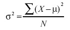
whereas the formula to estimate the variance from a sample is
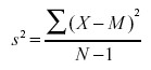
Notice that the denominators of the formulas are different: N for the population and N-1 for the sample. We saw in the “Estimating Variance Simulation” that if N is used in the formula for s2, then the estimates tend to be too low and therefore biased. The formula with N-1 in the denominator gives an unbiased estimate of the population variance. Note that N-1 is the degrees of freedom.
Sampling Variability – The sampling variability of a statistic refers to how much the statistic varies from sample to sample and is usually measured by its standard error ; the smaller the standard error, the less the sampling variability. For example, the standard error of the mean is a measure of the sampling variability of the mean. Recall that the formula for the standard error of the mean is

The larger the sample size (N), the smaller the standard error of the mean and therefore the lower the sampling variability.
Statistics differ in their sampling variability even with the same sample size. For example, for normal distributions, the standard error of the median is larger than the standard error of the mean. The smaller the standard error of a statistic, the more efficient the statistic. The relative efficiency of two statistics is typically defined as the ratio of their standard errors. However, it is sometimes defined as the ratio of their squared standard errors.
Estimation refers to the process by which one makes inferences about a population, based on information obtained from a sample. An estimate of a population parameter may be expressed in two ways, as
- Point estimate – A point estimate of a population parameter is a single value of a statistic. For example, the sample mean x is a point estimate of the population mean μ. Similarly, the sample proportion p is a point estimate of the population proportion P.
- Interval estimate – An interval estimate is defined by two numbers, between which a population parameter is said to lie. For example, a < x < b is an interval estimate of the population mean μ. It indicates that the population mean is greater than a but less than b.
