MapReduce Work Flow

Here are some of the key concepts related to MapReduce.

• Job – A Job in the context of Hadoop MapReduce is the unit of work to be performed as requested by the client / user. The information associated with the Job includes the data to be processed (input data), MapReduce logic / program / algorithm, and any other relevant configuration information necessary to execute the Job.
• Task – Hadoop MapReduce divides a Job into multiple sub-jobs known as Tasks. These tasks can be run independent of each other on various nodes across the cluster. There are primarily two types of Tasks – Map Tasks and Reduce Tasks.
• JobTracker – Just like the storage (HDFS), the computation (MapReduce) also works in a master-slave / master-worker fashion. A JobTracker node acts as the Master and is responsible for scheduling / executing Tasks on appropriate nodes, coordinating the execution of tasks, sending the information for the execution of tasks, getting the results back after the execution of each task, re-executing the failed Tasks, and monitors / maintains the overall progress of the Job. Since a Job consists of multiple Tasks, a Job’s progress depends on the status / progress of Tasks associated with it. There is only one JobTracker node per Hadoop Cluster.
• TaskTracker – A TaskTracker node acts as the Slave and is responsible for executing a Task assigned to it by the JobTracker. There is no restriction on the number of TaskTracker nodes that can exist in a Hadoop Cluster. TaskTracker receives the information necessary for execution of a Task from JobTracker, Executes the Task, and Sends the Results back to JobTracker.
• Map() – Map Task in MapReduce is performed using the Map() function. This part of the MapReduce is responsible for processing one or more chunks of data and producing the output results.
• Reduce() – The next part / component / stage of the MapReduce programming model is the Reduce() function. This part of the MapReduce is responsible for consolidating the results produced by each of the Map() functions/tasks.
• Data Locality – MapReduce tries to place the data and the compute as close as possible. First, it tries to put the compute on the same node where data resides, if that cannot be done (due to reasons like compute on that node is down, compute on that node is performing some other computation, etc.), then it tries to put the compute on the node nearest to the respective data node(s) which contains the data to be processed. This feature of MapReduce is “Data Locality”.

The following diagram shows the logical flow of a MapReduce programming model.

The stages depicted above are

• Input: This is the input data / file to be processed.
• Split: Hadoop splits the incoming data into smaller pieces called “splits”.
• Map: In this step, MapReduce processes each split according to the logic defined in map() function. Each mapper works on each split at a time. Each mapper is treated as a task and multiple tasks are executed across different TaskTrackers and coordinated by the JobTracker.
• Combine: This is an optional step and is used to improve the performance by reducing the amount of data transferred across the network. Combiner is the same as the reduce step and is used for aggregating the output of the map() function before it is passed to the subsequent steps.
• Shuffle & Sort: In this step, outputs from all the mappers is shuffled, sorted to put them in order, and grouped before sending them to the next step.
• Reduce: This step is used to aggregate the outputs of mappers using the reduce() function. Output of reducer is sent to the next and final step. Each reducer is treated as a task and multiple tasks are executed across different TaskTrackers and coordinated by the JobTracker.
• Output: Finally the output of reduce step is written to a file in HDFS.

Word Count Example

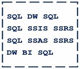
For the purpose of understanding MapReduce, let us consider a simple example. Let us assume that we have a file which contains the following four lines of text.

In this file, we need to count the number of occurrences of each word. For instance, DW appears twice, BI appears once, SSRS appears twice, and so on. Let us see how this counting operation is performed when this file is input to MapReduce.

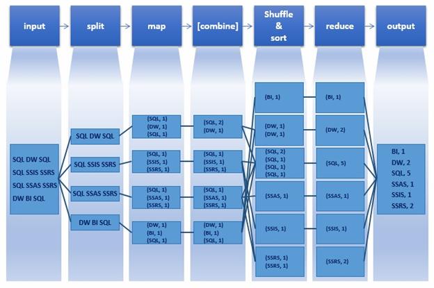
Below is a simplified representation of the data flow for Word Count Example.

• Input: In this step, the sample file is input to MapReduce.
• Split: In this step, Hadoop splits / divides our sample input file into four parts, each part made up of one line from the input file. Note that, for the purpose of this example, we are considering one line as each split. However, this is not necessarily true in a real-time scenario.
• Map: In this step, each split is fed to a mapper which is the map() function containing the logic on how to process the input data, which in our case is the line of text present in the split. For our scenario, the map() function would contain the logic to count the occurrence of each word and each occurrence is captured / arranged as a (key, value) pair, which in our case is like (SQL, 1), (DW, 1), (SQL, 1), and so on.
• Combine: This is an optional step and is often used to improve the performance by reducing the amount of data transferred across the network. This is essentially the same as the reducer (reduce() function) and acts on output from each mapper. In our example, the key value pairs from first mapper “(SQL, 1), (DW, 1), (SQL, 1)” are combined and the output of the corresponding combiner becomes “(SQL, 2), (DW, 1)”.
• Shuffle and Sort: In this step, output of all the mappers is collected, shuffled, and sorted and arranged to be sent to reducer.
• Reduce: In this step, the collective data from various mappers, after being shuffled and sorted, is combined / aggregated and the word counts are produced as (key, value) pairs like (BI, 1), (DW, 2), (SQL, 5), and so on.
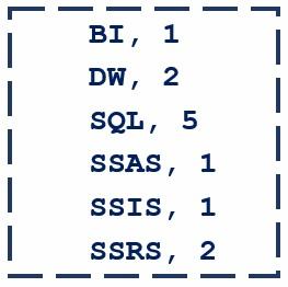
• Output: In this step, the output of the reducer is written to a file on HDFS. The following image is the output of our word count example.

Game Example

Say you are processing a large amount of data and trying to find out what percentage of your user base where talking about games. First, we will identify the keywords which we are going to map from the data to conclude that its something related to games. Next, we will write a mapping function to identify such patterns in our data. For example, the keywords can be Gold medals, Bronze medals, Silver medals, Olympic football, basketball, cricket, etc.

Let us take the following chunks in a big data set and see how to process it.

“Hi, how are you”

“We love football”

“He is an awesome football player”

“Merry Christmas”

“Olympics will be held in China”

“Records broken today in Olympics”

“Yes, we won 2 Gold medals”

“He qualified for Olympics”

Mapping Phase – So our map phase of our algorithm will be as

1. Declare a function “Map”
2. Loop: For each words equal to “football”
3. Increment counter
4. Return key value “football”=>counter

In the same way, we can define n number of mapping functions for mapping various words: “Olympics”, “Gold Medals”, “cricket”, etc.

Reducing Phase – The reducing function will accept the input from all these mappers in form of key value pair and then processing it. So, input to the reduce function will look like the following:

reduce(“football”=>2)

reduce(“Olympics”=>3)

Our algorithm will continue with the following steps

5. Declare a function reduce to accept the values from map function.
6. Where for each key-value pair, add value to counter.
7. Return “games”=> counter.

At the end, we will get the output like “games”=>5.

Now, getting into a big picture we can write n number of mapper functions here. Let us say that you want to know who all where wishing each other. In this case you will write a mapping function to map the words like “Wishing”, “Wish”, “Happy”, “Merry” and then will write a corresponding reducer function.

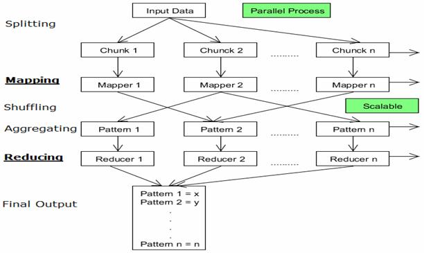
Here you will need one function for shuffling which will distinguish between the “games” and “wishing” keys returned by mappers and will send it to the respective reducer function. Similarly you may need a function for splitting initially to give inputs to the mapper functions in form of chunks. The following diagram summarizes the flow of Map reduce algorithm:

In the above map reduce flow

• The input data can be divided into n number of chunks depending upon the amount of data and processing capacity of individual unit.
• Next, it is passed to the mapper functions. Please note that all the chunks are processed simultaneously at the same time, which embraces the parallel processing of data.
• After that, shuffling happens which leads to aggregation of similar patterns.
• Finally, reducers combine them all to get a consolidated output as per the logic.
• This algorithm embraces scalability as depending on the size of the input data, we can keep increasing the number of the parallel processing units.