Maintainability is defined as the probability of performing a successful repair action within a given time. In other words, maintainability measures the ease and speed with which a system can be restored to operational status after a failure occurs. This is similar to system reliability analysis except that the random variable of interest in maintainability analysis is time-to-repair rather than time-to-failure. For example, if it is said that a particular component has a 90% maintainability for one hour, this means that there is a 90% probability that the component will be repaired within an hour. When you combine system maintainability analysis with system reliability analysis, you can obtain many useful results concerning the overall performance (availability, uptime, downtime, etc.) that will help you to make decisions about the design and/or operation of a repairable system.
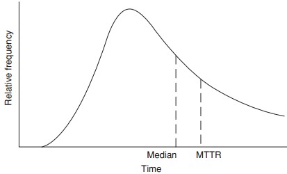
Maintenance times tend to be log normally distributed as shown by analysis of data. It also fits our experience and intuition that, for a task or group of tasks, there are occasions when the work is performed rather quickly, but it is relatively unlikely that the work will be done in much less time than usual, whereas it is relatively more likely that problems will occur which will cause the work to take much longer than usual. This skews time-to-repair distributions to the right.

In addition to the job-to-job variability, leading typically to a lognormal distribution of repair times, there is also variability due to learning. Depending upon how data are collected, this variability might be included in the job-to-job variability, for example if technicians of different experience are being used simultaneously. However, both the mean time and the variance should reduce with experience and training.
Usually a system can be restored to an operational state rather quickly after a given failure occurs or a given maintenance action is required. There is some probability that problems will occur that cause the downtime to be quite lengthy. The distribution models the time to perform the action and the probability that the action will be necessary. The probability density function of the lognormal is

The mean of the lognormal is

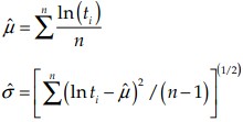
If the data are distributed as a lognormal distribution, the natural logarithms of the data are distributed as a normal distribution. m is not the mean of the lognormal data, but is the mean of the loge of the data. s is the standard deviation of the loge of the data. The estimates of the distribution parameters from sample data are

The Weibull distribution can also be used to model times to repair. The Weibull distribution peaks near the origin and is then skewed to the right for shape parameters in a range of 1.2 to 2.0.

