A hypothesis is a theory about the relationships between variables. Statistical analysis is used to determine if the observed differences between two or more samples are due to random chance or to true differences in the samples.
Terminology
A hypothesis is a value judgment, a statement based on an opinion about a population. It is developed to make an inference about that population. Based on experience, a design engineer can make a hypothesis about the performance or qualities of the products she is about to produce, but the validity of that hypothesis must be ascertained to confirm that the products are produced to the customer’s specifications. A test must be conducted to determine if the empirical evidence does support the hypothesis.
Null Hypothesis – The first step consists in stating the hypothesis. It is denoted by H0, and is read “H sub zero.” The statement will be written as H0: µ = 20%. A null hypothesis assumes no difference exists between or among the parameters being tested and is often the opposite of what is hoped to be proven through the testing. The null hypothesis is typically represented by the symbol Ho.
Alternate Hypothesis – If the hypothesis is not rejected, exactly 20 percent of the defects will actually be traced to the CPU socket. But if enough evidence is statistically provided that the null hypothesis is untrue, an alternate hypothesis should be assumed to be true. That alternate hypothesis, denoted H1, tells what should be concluded if H0 is rejected. H1 : µ ≠ 20%. An alternate hypothesis assumes that at least one difference exists between or among the parameters being tested. This hypothesis is typically represented by the symbol Ha.

Test Statistic – The decision made on whether to reject H0 or fail to reject it depends on the information provided by the sample taken from the population being studied. The objective here is to generate a single number that will be compared to H0 for rejection. That number is called the test statistic. To test the mean µ, the Z formula is used when the sample sizes are greater than 30,
and the t formula is used when the samples are smaller,

The level of risk – It addresses the risk of failing to reject a hypothesis when it is actually false, or rejecting a hypothesis when it is actually true.
Type I error (False Positive) – It occurs when one rejects the null hypothesis when it is true. The probability of a type I error is the level of significance of the test of hypothesis, and is denoted by *alpha*. Usually a one-tailed test of hypothesis is used when one talks about type I error or alpha error.
Type II error (False Negative) – It occurs when one rejects the alternative hypothesis (fails to reject the null hypothesis) when the alternative hypothesis is true. The probability of a type II error is denoted by *beta*. One cannot evaluate the probability of a type II error when the alternative hypothesis is of the form µ > 180, but often the alternative hypothesis is a competing hypothesis of the form: the mean of the alternative population is 300 with a standard deviation of 30, in which case one can calculate the probability of a type II error.
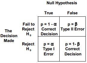
Decision Rule Determination – The decision rule determines the conditions under which the null hypothesis is rejected or not. The critical value is the dividing point between the area where H0 is rejected and the area where it is assumed to be true.
Decision Making – Only two decisions are considered, either the null hypothesis is rejected or it is not. The decision to reject a null hypothesis or not depends on the level of significance. This level often varies between 0.01 and 0.10. Even when we fail to reject the null hypothesis, we never say “we accept the null hypothesis” because failing to reject the null hypothesis that was assumed true does not equate proving its validity.
Testing for a Population Mean – When the sample size is greater than 30 and σ is known, the Z formula can be used to test a null hypothesis about the mean. The Z formula is as

Phrasing – In hypothesis testing, the phrase “to accept” the null hypothesis is not typically used. In statistical terms, the Six Sigma Black Belt can reject the null hypothesis, thus accepting the alternate hypothesis, or fail to reject the null hypothesis. This phrasing is similar to jury’s stating that the defendant is not guilty, not that the defendant is innocent.
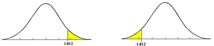
One Tail Test – In a one-tailed t-test, all the area associated with a is placed in either one tail or the other. Selection of the tail depends upon which direction to bs would be (+ or -) if the results of the experiment came out as expected. The selection of the tail must be made before the experiment is conducted and analyzed.
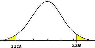
Two Tail Test – If a null hypothesis is established to test whether a population shift has occurred, in either direction, then a two tail test is required. The allowable a error is generally divided into two equal parts.
Statistical vs Practical Significance
Practical Significance – Practical significance is the amount of difference, change or improvement that will add practical, economic or technical value to an organization.
Statistical Significance – Statistical significance is the magnitude of difference or change required to distinguish between a true difference, change or improvement and one that could have occurred by chance. The larger the sample size, the more likely the observed difference is close to the actual difference.
To achieve victory in a project, both practical and statistical improvements are required. It is possible to find a difference to be statistically significant but not of practical significance. Because of the limitations of cost, risk, timing, etc., project team cannot implement practical solutions for all statistically significant Xs. Determining practical significance in a Six Sigma project is not the responsibility of the Black Belt alone. Project team need to collaborate with others such as the project sponsor and finance manager to help determine the return on investment
(ROI) associated with the project objective.
Sample Size
It has been assumed that the sample size (n) for hypothesis testing has been given and that the critical value of the test statistic will be determined based on the a error that can be tolerated. The sample size (n) needed for hypothesis testing depends on the desired type I (a) and type II (b ) risk, the minimum value to be detected between the population means (m – m0) and the variation in the characteristic being measured (S or s).
Point and Interval Estimates
Estimation refers to the process by which one makes inferences about a population, based on information obtained from a sample. An estimate of a population parameter may be expressed in two ways, as
- Point estimate – A point estimate of a population parameter is a single value of a statistic. For example, the sample mean x is a point estimate of the population mean μ. Similarly, the sample proportion p is a point estimate of the population proportion P.
- Interval estimate – An interval estimate is defined by two numbers, between which a population parameter is said to lie. For example, a < x < b is an interval estimate of the population mean μ. It indicates that the population mean is greater than a but less than b.
Unbiased Estimator – When the mean of the sampling distribution of a statistic is equal to a population parameter, that statistic is said to be an unbiased estimator of the parameter. If the average estimate of several random samples equals the population parameter, the estimate is unbiased. For example, if credit card holders in a city were repetitively random sampled and questioned what their account balances were as of a specific date, the average of the results across all samples would equal the population parameter. If however, only credit card holders in one neighborhood were sampled, the average of the sample estimates would be a biased estimator of all account balances for the city and would not equal the population parameter.
Efficient Estimator – It is an estimator that estimates the quantity of interest in some “best possible” manner. The notion of “best possible” relies upon the choice of a particular loss function — the function which quantifies the relative degree of undesirability of estimation errors of different magnitudes. The most common choice of the loss function is quadratic, resulting in the mean squared error criterion of optimality.
Prediction Interval – It is an estimate of an interval in which future observations will fall, with a certain probability, given what has already been observed. Prediction intervals are often used in regression analysis.
Tests for means, variances and proportions
Confidence Intervals for the Mean – The confidence interval for the mean for continuous data with large samples is

where, ![]() is the normal distribution value for a desired confidence level. If a relatively small sample is used (<30) then the t distribution must be used. The confidence interval for the mean for continuous data with small samples is
is the normal distribution value for a desired confidence level. If a relatively small sample is used (<30) then the t distribution must be used. The confidence interval for the mean for continuous data with small samples is

The ![]() distribution value for a desired confidence level,
distribution value for a desired confidence level, ![]() uses (n – 1) degrees of freedom.
uses (n – 1) degrees of freedom.
Confidence Intervals for Variation – The confidence intervals for variance is based on the Chi-Square distribution. The formula is
S2 is the point estimate of variance and ![]() are the chi-square table values for (n – 1) degrees of freedom
are the chi-square table values for (n – 1) degrees of freedom
Confidence Intervals for Proportion – For large sample sizes, with n(p) and n(1-p) greater than or equal to 4 or 5, the normal distribution can be used to calculate a confidence interval for proportion. The following formula is used
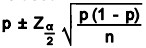
![]() is the appropriate confidence level from a Z table.
is the appropriate confidence level from a Z table.
Population Variance – The confidence interval equation is as 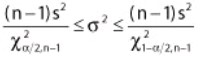
Population Standard Deviation – The equation is 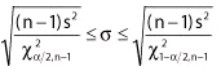
The statistical tests for means usually are
- One-sample Z-test: for population mean
- Two-sample Z-test: for population mean
- One-sample T-test: single mean (one sample versus historic mean or target value)
- Two-sample T-test : multiple means (sample from each of the two categories)
One-Sample Z-Test for Population Mean – The One-sample Z-test for population mean is used when a large sample (n≥ 30) is taken from a population and we want to compare the mean of the population to some claimed value. This test assumes the population standard deviation is known or can be reasonably estimated by the sample standard deviation and uses the Z distribution. Null hypothesis is Ho: μ = μ0 where, μ0 is the claim value compared to the sample.
Two-Sample Z-Test for Population Mean – The Two-sample Z-test for population mean is used after taking 2 large samples (n≥30) from 2 different populations in order to compare them. This test uses the Z-table and assumes knowing the population standard deviation, or estimated by using the sample standard deviation. Null hypothesis is Ho: μ1= μ2
One-Sample T-test – The One-sample T-test is used when a small sample (n< 30) is taken from a population and to compare the mean of the population to some claimed value. This test assumes the population standard deviation is unknown and uses the t distribution. The null hypothesis is Ho: μ = μ0 where μ0 is the claim value compared to the sample. The test statistic is

where x is the sample mean, s is the sample standard deviation and n is the sample size.
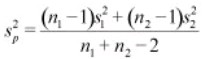
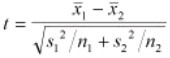
Two-Sample T-test – The Two-sample T-test is used when two small samples (n< 30) are taken from two different populations and compared. There are two forms of this test: assumption of equal variances and assumption of unequal variances. The null hypothesis is Ho: µ1= µ2. The Test Statistic with assumption of equal variances is
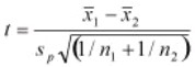
Where pooled variance is
Taking assumption of unequal variances then the test statistic is as
Analysis of Variance (ANOVA)
Sometimes it is essential to compare three or more population means at once with the assumptions as the variance is the same for all factor treatments or levels, the individual measurements within each treatment are normally distributed and the error term is considered a normally and independently distributed random effect. With analysis of variance, the variations in response measurement are partitioned into components that reflect the effects of one or more independent variables. The variability of a set of measurements is proportional to the sum of squares of deviations used to calculate the variance ![]() .
.
Analysis of variance partitions the sum of squares of deviations of individual measurements from the grand mean (called the total sum of squares) into parts: the sum of squares of treatment means plus a remainder which is termed the experimental or random error.
ANOVA is a technique to determine if there are statistically significant differences among group means by analyzing group variances. An ANOVA is an analysis technique that evaluates the importance of several factors of a set of data by subdividing the variation into component parts. ANOVA tests to determine if the means are different, not which of the means are different Ho: μ1= μ2= μ3 and Ha: At least one of the group means is different from the others.
ANOVA extends the Two-sample t-test for testing the equality of two population means to a more general null hypothesis of comparing the equality of more than two means, versus them not all being equal.
One-Way ANOVA
Terms used in ANOVA
- Degrees of Freedom (df) – The number of independent conclusions that can be drawn from the data.
- SSFactor – It measures the variation of each group mean to the overall mean across all groups.
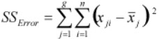
- SSError – It measures the variation of each observation within each factor level to the mean of the level.
- Mean Square Error (MSE) – It is SSError/ df and is also the variance.
- F-test statistic – The ratio of the variance between treatments to the variance within treatments = MS/MSE. If F is near 1, then the treatment means are no different (p-value is large).
- P-value – It is the smallest level of significance that would lead to rejection of the null hypothesis (Ho). If α = 0.05 and the p-value ≤ 0.05, then reject the null hypothesis and conclude that there is a significant difference and if α = 0.05 and the p-value > 0.05, then fail to reject the null hypothesis and conclude that there is not a significant difference.
One-way ANOVA is used to determine whether data from three or more populations formed by treatment options from a single factor designed experiment indicate the population means are different. The assumptions in using One-way ANOVA is all samples are random samples from their respective populations and are independent, distributions of outputs for all treatment levels follow the normal distribution and equal or homogeneity of variances.
Steps for computing one-way ANOVA are
- Establish the hypotheses. Ho: μ1= μ2= μ3 and Ha: At least one of the group means is different from the others.
- Calculate the test statistic. Calculate the average of each call center (group) and the average of the samples.
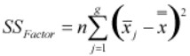
Calculate SSFactor as
Calculate SSError as
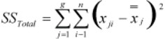
- Calculate SSTotal as
- Calculate the ANOVA table with degrees of freedom (df) is calculated for the group, error and total sum of squares.
- Determine the critical value. Fcritical is taken from the F distribution table.
Draw the statistical conclusion. If Fcalc< Fcritical fail to reject the null hypothesis and if Fcalc > Fcritical, reject the null hypothesis.
Chi Square Tests
Usually the objective of the project team is not to find the mean of a population but rather to determine the level of variation of the output like to know how much variation the production process exhibits about the target to see what adjustments are needed to reach a defect-free process.
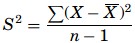
If the means of all possible samples are obtained and organized we can derive the sampling distribution of the means similarly for variances, the sampling distribution of the variances can be known but, the distribution of the means follows a normal distribution when the population is normally distributed or when the samples are greater than 30, the distribution of the variance follows a Chi square (χ2) distribution. As the sample variance is computed as
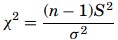
Then the χ2 formula for single variance is given as
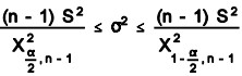
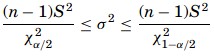
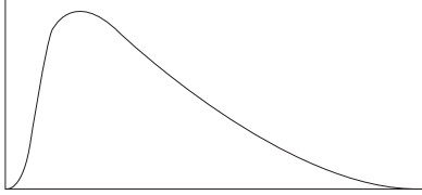
The shape of the χ2 distribution resembles the normal curve but it is not symmetrical, and its shape depends on the degrees of freedom. The χ2 formula can be rearranged to find σ2. The value σ2 with a degree of freedom of n−1, will be within the interval
The chi-square test compares the observed values to the expected values to determine if they are statistically different when the data being analyzed do not satisfy the t-test assumptions. The chi-square goodness-of-fit test is a non-parametric test which compares the expected frequencies to the actual or observed frequencies. The formula for the test is
with fe as the expected frequency and fa as the actual frequency. The degree of freedom will be given as df= k − 1. Chi-square cannot be negative because it is the square of a number. If it is equal to zero, all the compared categories would be identical, therefore chi-square is a one-tailed distribution. The null and alternate hypotheses will be df= k − 1.
Chi-square cannot be negative because it is the square of a number. If it is equal to zero, all the compared categories would be identical, therefore chi-square is a one-tailed distribution. The null and alternate hypotheses will be H0: The distribution of quality of the products after the parts were changed is the same as before the parts were changed. H1: The distribution of the quality of the products after the parts were changed is different than it was before they were changed.
