There are two basic approaches to the problem of sample size – the ad hoc or practical approach and the statistical approach The former is widely used in marketing research.
Practical Method: According to this approach, a sample size of less than a few hundred units is not chosen. This is because when a field survey is undertaken, interviewers are appointed, trained and asked to conduct field investigations. Since all this would cost substantially, it would not be worth it for the marketing researcher if only a small sample is chosen. A survey confined to a relatively small number of units would mean a relatively high cost per interview. Another consideration in favour of selecting a reasonable size of sample is that it enables that researcher to test several hypotheses. This is especially true for samples in the sub-groups. Such hypotheses can be tested with a high degree of statistical significance when the sample size is reasonable large. Another practical consideration in case of a stratified sample is that the overall sample size is so fixed that the sample size within each stratum is not less than 30. A common practice in this regard is to determine the sample size of each stratum first and then add up the samples of all the strata to obtain the overall sample size.
Statistical Principles: The second approach based on statistical principles is obviously scientific. A good researcher is expected to follow it rather than the rule-of-thumb approach. According to the statistical approach, the problem of sample size involves several aspects such as the type of sample design, the homogeneity in the population from which a sample is to be chosen and the availability of finance, personnel and time for the conduct of the field survey. In view of all these considerations, the question of sample size becomes difficult. Since a comprehensive discussion of all these aspects would need a good deal of space, only some basic principles for determining sample size are discussed.
However, before this is done, it is necessary to have some idea of sampling distribution, which forms the basis for any problem on sample size.
Sampling Distribution of the Mean: According to the central limit theorem, the various arithmetic means of a large number of random samples of the same size will form a normal distribution. If an arithmetic mean of all possible sample means is calculated, it will coincide with the population mean. To illustrate this point, let us take a sample example:
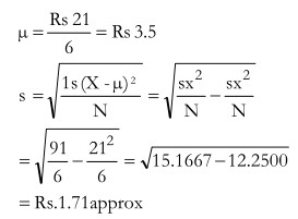
Suppose there are six persons A, B, C, D, E and F constituting the population. Each one of them has some money. Assume that A has rupee one, B rupees two, and so on. Then, the population means and standard deviation will be as follows:
| Identity of persons | Amount (X) | X2 |
| A | 1 | 1 |
| B | 2 | 4 |
| C | 3 | 9 |
| D | 4 | 16 |
| E | 5 | 25 |
| F | 6 | 36 |
| ——- 21 | —– 91 |
Suppose two persons are selected as a sample. The number of possible sample size 2 that can be selected is:
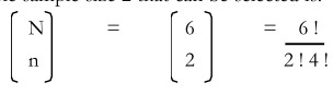
(Total number of samples without replacement)
| S.No. | Sample | Sample Mean |
| 1 | A, B | 1.5 |
| 2 | A, C | 2.0 |
| 3 | A, D | 2.5 |
| 4 | A, E | 3.0 |
| 5 | A, F | 3.5 |
| 6 | B, C | 2.5 |
| 7 | B, D | 3.0 |
| 8 | B, E | 3.5 |
| 9 | B, F | 4.0 |
| 10 | C, D | 3.5 |
| 11 | C, E | 4.0 |
| 12 | C, F | 4.5 |
| 13 | D, E | 4.5 |
| 14 | D, F | 5.0 |
| 15 | E, F | 5.5 |
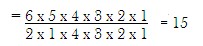
Tables below show the distribution of sample means, as also some other calculations.
| Sample Mean | Frequency | Deviation from assumed mean = 4 | d÷0.5 | Fd | D2 | Fd2 |
| .5 | 1 | – 2.5 | – 5 | – 5 | 25 | 25 |
| 2.0 | 1 | – 2.0 | – 4 | – 4 | 16 | 16 |
| 2.5 | 2 | – 1.5 | – 3 | – 6 | 9 | 18 |
| 3.0 | 2 | – 1.0 | – 2 | – 4 | 4 | 8 |
| 3.5 | 3 | – 0.5 | – 1 | – 3 | 1 | 3 |
| 4.0 | 2 | 0 | 0 | 0 | 0 | 0 |
| 4.5 | 2 | 0.5 | 1 | 2 | 1 | 2 |
| 5.0 | 1 | 1.0 | 2 | 2 | 4 | 4 |
| 5.5 | 1 | 1.5 | 3 | 3 | 9 | 9 |
| ——– 15 | —– -22 +7 —— -15 | —– 69 | —- 85 |
There is a certain relationship between the two. This is best explained by the following formula:
Where σx = standard error of the sample distribution
σ = Standard deviation of the population
n = sample size
N = Number of units in the population
Where σx = standard error of the sample distribution σ = Standard deviation of the population n = sample size N = Number of units in the population
Applying the different values in the above formula
= 1.08 (same as obtained earlier)
The term is called the finite population correction (fpc). It may be noted that in case of an infinite population, the term
![]() approaches 1.00 and hence the finite population correction also approaches 1.00. In such a case, the formula become
approaches 1.00 and hence the finite population correction also approaches 1.00. In such a case, the formula become ![]() In the case of sampling with replacement, there is an infinite population and as such, the reduced version of the formula may be used. In other cases too, if the sample is relatively too small vis-à-vis the population, fpc need not be used as it will approach 1.00. In other words, when N is large relative to n, formula
In the case of sampling with replacement, there is an infinite population and as such, the reduced version of the formula may be used. In other cases too, if the sample is relatively too small vis-à-vis the population, fpc need not be used as it will approach 1.00. In other words, when N is large relative to n, formula ![]() may be used. The question is: how to decide that N is relatively larger than n? Different people may take different values but the general practice is to use this formula (which excludes the correction factor) when n is less than 5 per cent of N.
may be used. The question is: how to decide that N is relatively larger than n? Different people may take different values but the general practice is to use this formula (which excludes the correction factor) when n is less than 5 per cent of N.
Characteristics of the Distribution of Sample Means
- Although the population shows a rectangular distribution, the distribution of sample means shows a symmetrical distribution and has only one mode, i.e. it is unimodal.
- The mean of the sample distribution coincides with the mean of the population. In the example given above, the population mean is Rs.3.5 (Table 10.1) and the mean of the distribution of the sample means too happens to be Rs.3.5 (Table 10.3).
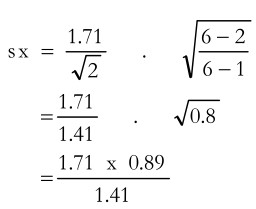
- The standard deviation of the population, and the standard deviation of the sample means, sx, is related, as is indicated by the formula given earlier. If the finite population correction is to be ignored, then the standard deviation of the distribution of sample means n s sx = It may be noted that sx (Table 10.3) was 1.08 whereas s (Table 10.1) was 1.71).
In other words, the standard deviation of the sample means turns out to be smaller than that of the population. Further, it may be noted that the former tends to be smaller as the sample size, n, increases. This is because of the fact that as the sample size increase, the mean of the sample distribution tends to be closer to the population mean which, in turn, makes the scatter of the sample means narrower.
Since the formula for the relationship between the standard deviation of the population and the standard error of the
Sample is 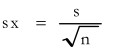 we find that
  ignoring the finite population correction.
Thus, to determine n, the size of the sample, both the numerator and the denominator should be known to us.
Main Consideration for Sample Size Decisions
There are three consideration required to be checked when determining the sample size necessary to estimate the population mean. These are
- The extent of error or imprecision allowed.
- The degree of confidence desired in the estimate.
- Estimate of the standard deviation of the population.
The first two considerations involve the judgment of the researcher. The third consideration is the responsibility of the researcher. Sometimes estimates of standard deviation are available, from earlier studies. Even when standard deviation is not available, it can be calculated from the summary tables containing the data. However, if this too is not possible, the researcher may choose a small sample from which the standard deviation is calculated. He then uses the sample standard deviation as an estimate of the population standard deviation and then determines and final sample size. The initial sample need not be discarded afterwards and can be used as a part of the final sample. However, some additional time is needed to carry out this exercise.
We may consider the problem of determining sample size in two different situations, namely when the standard deviation of the population is known and when it is unknown.
Determination of sample size when standard deviation is known
Extent of Error: The first consideration relates to the extent of error allowed. This is indicated by the standard error (i.e. the standard deviation of the sample means). The researcher himself has to decide the magnitude of the standard error that he can tolerate. Although this is a difficult question, it is necessary to fix the limit of the standard error beyond which it should not exceed. The fixation of standard error should not be confined to overall results but should also be applied to various sub-groups. One way is to first determine the size of each sub-group on the basis of a given degree of precision. The total of the size of each sub-group could then be taken as the overall size of the sample, though it may turn out to be too large and on considerations of time and money, it may not be acceptable to the researcher.
The Degree of Confidence: A second consideration is the degree of confidence that the researcher wants to have in the results of the study. In case he wants to be 100 per cent confident of the results, he is left with no option but the to cover the entire population. However, as this is often not possible on account of cost, time and other constraints, the researcher should be satisfied with less then 100 per cent confidence. Normally, three confidence levels, namely, 99 per cent, 95 per cent and 90 per cent are used. When a 99 per cent confidence level is used, it implies that there is a risk of only 1 per cent of the true population statistic falling outside the range indicated by the confidence interval. In the case of a 95 per cent confidence level, such a risk is of 5 per cent and in the case of 90 per cent confidence level, it is of 10 per cent. In marketing research studies, the most frequently used norm is the 5 per cent confidence level.
It should be noted that there is a trade off between the degree of precision and the degree of confidence. For a given size of a sample, one can specify one of these two but not both of them at the same time. To illustrate this point, let us assume that in a survey of households in a certain territory, the average income per household has turned out to be Rs.1000 per month. As this is a point estimate, it is not associated with any bounds of error and, therefore, it is regarded as a precise estimate. At the same time, such an estimate is likely to be wrong, i.e. one can associate a very low level of confidence with it. In contract, if we say that the average monthly income per household varies from Rs.500 to Rs.2500, we are associating a very high degree of confidence in this estimate, although it tends to be far less precise than the earlier one. An estimate of this type, having a very wide range, will not be of much help to the researcher.
The foregoing basic considerations involved in determining the sample size can be better understood with the help of some examples. We have earlier seen the sampling distribution of sample means. According to the Central Limit Theorem, the distribution of sample means will be normal regardless of the distribution of population.
Let us first take the case where the population variance is known. Suppose in our previous example of average monthly income per household, we find that the standard deviation is Rs.100. Further, we suppose that the estimate in within ± Rs.40 of the true population mean. This means that the total precision is 80 and half precision is 40. We shall use the latter value, as we shall work out the calculations on the basis of one-half of the curve. In this way, certain calculations can be simplified as we know that the populations mean m divides the normal curve into two equal halves.
Another point that needs to be decided relates to the degree of confidence in the result that one would like to have. Suppose that this degree of confidence is 95 per cent which would imply that Z is approximately 2. Strictly speaking, the 95 per cent confidence interval gives Z = 1.96 which can be taken as 2 so as to simplify the calculations.
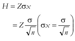
The formula is determined the size of n is:
where H is half precision which is 40 in the above example; Z = 2 approximately and s is 100.
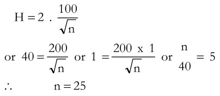
This calculation given the sample size as 25 This indicates that when the standard deviation of population is Rs.100 and the extent of precision in Rs.40, a sample of 25 households needs to be chosen.
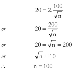
Let us take a few more examples, making certain variations in the original values. Suppose that we are interested in making out estimate twice as precise as the earlier one, then H becomes 20 instead of 40. Taking Z = 2 and standard deviation as 100, as in the earlier case, and applying the formula ![]() we get
we get
We find that the value of n now arrived at is 100, i.e., four times of the original value. In other words, when precision is doubled, the value of n increases four times. This result can be generalised as follows: When the precision is increased by a factor x, sample size increases by a factor x2.
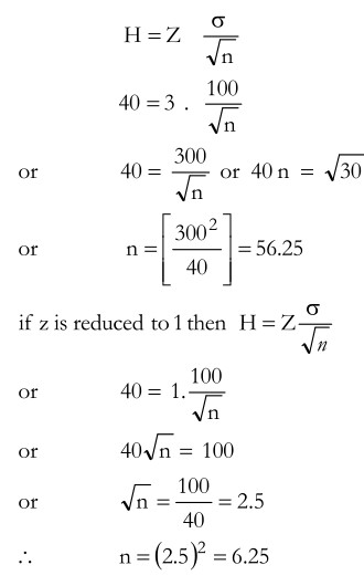
Let us now see what happens to the sample size n if the degree of confidence undergoes a change. Suppose that the degree of confidence is 99 per cent instead of 95 per cent, then Z is equal to 3. Thus
Notice the changes in the value of n. In the first case, when Z is increased from 2 to 3, there is an increase of 3/2 times in its value. When Z is increased 3/2 time, the value of n increases 3/2 X 3/2 = 9/4 times as 25 X 9/4 = 225/4 = 56.25 Likewise, when the value of Z is reduced from 2 to 1, there is a fall in its value by 1/2. When Z is reduced by 1/2, the value of n reduces to 1/2 X 1/2 X 1/4 th of its original value n = 25 25 = 2 2 4 4 6.25. To generalise the above results, when Z is increased by a certain factor y, sample size increases by a factor y2.
When Standard Deviation of Population is Unknown
So far the discussion was confined to such cases where standard deviation of the population was known. May a time, the standard deviation is not known. In such cases too, the method followed is the same except that an estimate of the population standard deviation in place of its previously known value is taken. Sometimes, the researcher may undertake a pilot survey to ascertain the standard deviation. If this is not possible, the researcher may have to use some alternative approach. As we know, the entire area under the normal curve falls within µ ± 3σ. This means that we should have some idea of the range of variation, i.e. the difference between the highest item and the lowest item.
Suppose in our previous example, the minimum monthly income amongst households is Rs.500 and the maximum is Rs.2000. This gives a range of Rs.1500 which divided by 6 yields a figure of 250. This is the estimated value of σ. Taking other values as earlier, the sample size can be determined as shown below.
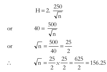
This shows that a sample of 156 households should be taken. Suppose a sample of 156 households gives a sample mean X = 1000, and a sample standard deviation Š = 200, then the confidence interval would be X ± ZSx
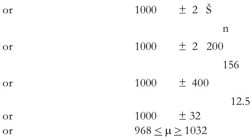
This shows the precision as ± 32 as against ± 40 in the earlier example. Thus the interval has become narrower than earlier envisaged. This is because the sample standard deviation (200) is less than the estimated population standard deviation (250) in the earlier example. In other words, as the population standard deviation was over-estimated as judged by the sample standard deviation, the confidence interval became narrower. Conversely, if the population standard deviation turns out to be under-estimated vis-à-vis sample standard deviation, the confidence interval will become wider.
Relative Precision: So far the discussion was concerned with the basis of absolute precision measured in terms of specific units. We now introduce another dimension, namely, the relative precision. It can be defined as the extent of precision relative to level. Suppose the mean is 200 and a relative precision of 10 per cent is aimed at. This would mean a confidence interval from 180 to 220. In case the mean is 100, the confidence interval will be from 90 to 110.
When applying relative precision instead of absolute precision, the usual formula![]() is transformed to
is transformed to ![]() where = r the n n relative precision and m is the mean of the population. This, too, can be changed as shown below.
where = r the n n relative precision and m is the mean of the population. This, too, can be changed as shown below.
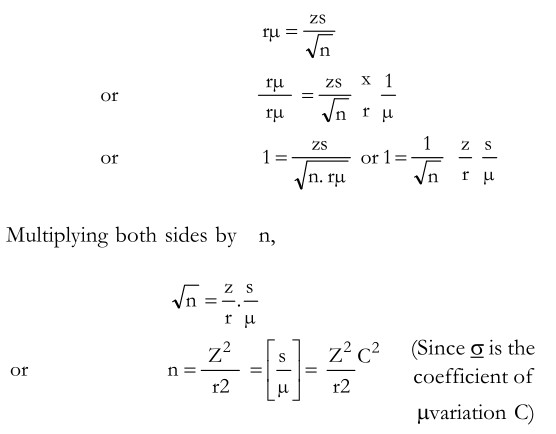
In the above form of the formula, it is necessary to have values of three variable namely, z, r and C. Since Z relates to the desired level of significance, it will be known. So also r will be known as it indicates the level of precision which has to be decided in advance. It is only C that is not known and which needs to be estimated. The researcher has to very carefully use his judgment regarding the magnitudes of the population mean and the population standard deviation. If there are some earlier studies available for his guidance, he should draw upon them in order to make his judgment as realistic as possible. It may be noted that if the coefficient of variation C turns out to be higher than that actually given by the ratio of the sample standard deviation to the sample mean, then this would show that the sample size should have been larger and vice versa.
Cost as a Factor in Determining Sample Size: So far we have not considered cost, an important factor in determining sample size. However, cost is an important factor that influences sample size. Suppose a firm has earmarked a sum of Rs. 50, 000 for a research study involving field survey. It has also decided to choose a sample of 1200 respondents for a specified level of precision and 95 per cent confidence of the results. The study would involve several aspects such as training of interviewers, designing of questionnaires, supervision of field work, coding, editing and tabulation of collected data, analysis of data and report writing. Suppose further that the fixed costs are likely to be Rs.30, 000 and the field survey would cost Rs.20 per interview. In such a case, a sum of Rs.20, 000 (Rs.50,000 – Rs.30,000) is available for the field survey. Since one interview cost Rs.20, the field survey can cover Rs.20, 000 / Rs.20 i.e., 1000 respondents only. Thus the firm finds that the sample size of 1200 would not be possible. Now, the sample size of 1000 respondents would yield a lower degree of confidence, say, 90 per cent instead of 95 per cent as originally envisaged. The firm should, therefore, decide whether it would really serve its purpose.
Another alternative before the firm is to increase the size of the allowance error. A lower degree of precision would need a lower sample size than the 1200 determined earlier. Thus, one would notice that there could be several combinations of the extent of confidence and precision which can be thought of by the firm. It has to choose one of these feasible combinations, within the financial resources available. It may as well find that lowering of the degree of confidence or precision or both may considerably reduce the utility of the study. In such a case it may even go to other extreme and drop the idea of undertaking it.
Several Objectives: It should be noted that a marketing research study is seldom conducted to estimate a single parameter. Generally several objectives are involved in a single study. Now, a sample size may vary from one objective to another on account of the expected variance. It is not necessary to go through the process of determining sample size for all objectives. The general approach is to choose a few crucial questions on the basis of which the sample size is determined. The researcher should especially include objectives that are likely to have greater variability as their inclusion will be more crucial for sample size.
Suppose that in a study three parameters are to be estimated each with a 95 per cent confidence and within desired precision. The sample size required has been determined as 40 units, 80 units and 25 units, respectively. The most conservative approach in such a case would be to select a sample of 80 units, which is the largest. However, if the second parameter where sample size required is 80 is not crucial, it is advisable not to choose a sample of 80 units. Taking a sample of this size would involve additional expenditure which could be saved. In such a case a sample size of 40 would be most appropriate. Thus, the marketing researcher should be guided by the relative importance of the parameter and the one which is most crucial should be taken into consideration. The sample size should then be determined for the desired precision and confidence with respect to that parameter. The sample size thus determined should be applicable to the entire study, covering all the parameters.
In our preceding example, if a sample of 80 is chosen, then the degree of confidence as also precision will be higher than the desired degrees, as envisaged earlier. Conversely, if a lower sample size say, 25 units is chosen, then in case of the other two parameters, the degrees of confidence and precision would be lower than the corresponding values envisaged earlier. The researcher has to exercise his judgment very carefully in such cases.
Sample Size Decisions When Estimating Proportions: The foregoing discussion was carried out in relation to sample size for estimating mean values. At times, it is the proportion of population with a particular attribute that becomes more relevant to the marketing researcher than the mean value. For example, one may be more interested in knowing the proportion of households having a monthly income of, say, Rs.1000 and less or of Rs.2500 and above rather than in knowing the average income of the households.
The formula for the standard error of a proportion p based on a simple random sample of size n is
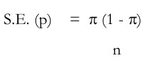
where p is the proportion of units with a particular attribute The above formula can be transformed as follows:
From the above formula, it is clear that the values of p and the standard error of a proportion should be known in order to determine the sample size, n. However, one finds that p is generally not known, which necessitates its estimation. Suppose the value of p is estimated so also the extent of the standard error is chosen, then one can arrive at the sample size. Further suppose that the sample size thus determined turns out to be a sizeable proportion of the population. In that case, it is necessary to use the finite population connection (fpc). This can be done with the help of the following formula
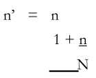
Where n’ is the revised size of the sample, n is the earlier size of the sample and N is the population size. Let us illustrate this. Suppose we are interested in estimating the proportion of households having a television set. We believe that this figure is about 20 per cent. Further, we decide that a standard error should not be more than 2 per cent. We now apply the earlier formula, namely,
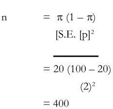
This gives the sample size of 400 households. This could be regarded as the desirable sample provided that the population is relatively large. It, however, population is only 1600 households, then the revised sample size can be worked out as follows:
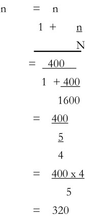
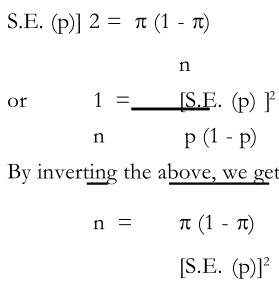
This shows that a sample size of 320 households should be taken instead of 400 households. From the formula
it should be clear that the value of π (1-π) would influence the size of n. The smaller is this value, the smaller will be the sample size required for a given standard error. It may also be noted that n will be at a maximum when p (1-π) is at a maximum. When π = 1/2, π(1-π) is at a maximum. This also shows that if a small standard error is to be preferred, then a relatively large sample size is required.
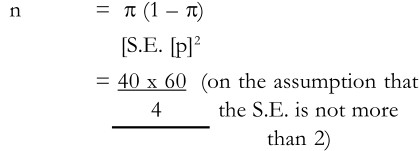
Another point that needs to be emphasised is that in the initial stage when an estimate of p is made, it may not be right. Let us take an example. Suppose the proportion of households earning Rs.1000 or less per month has been estimated as 0.40.
This means that 2400/4 = 600
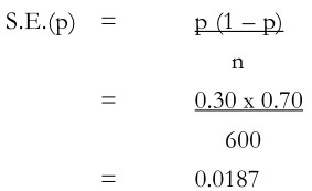
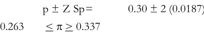
Suppose that when the survey is undertaken and the 600 sampled households are contacted, the sample proportion p turn out to be 0.30. With this revised proportion, the standard error is determined S.E.(p) = p (1 – p) n = 0.30 x 0.70 600 = 0.0187 and the confidence interval will then be p ± Z Sp= 0.30 ± 2 (0.0187) 0.263 < π > 0.337
The interval is narrower than desired as the sample proportion (0.30) turned out to be less than the population (0.40).
turn out to be 0.30. With this revised proportion, the standard error is determined
and the confidence interval will then be
Relative Precision: As was discussed earlier, while determining sample size when estimating means, here to the same approach is applicable in respect of relative precision The term ‘relative precision’ signifies that the size of the interval will be within a certain percent of the value, regardless of its level. For example, if the sample proportion is 0.40 and if the relative precision is to be within ± 10 per cent, then the interval would be 0.36 to 0.44.
Statistical Efficiency: The term ‘efficiency’ or statistical efficiency’ is frequently used in discussions of sampling. A sample design is considered statistically more efficient than another if its standard error of the mean is smaller, given the same sample size. Conversely, a more efficient sample design will yield as precise a result as an alternative sample design but with a smaller sample. Thus, efficiency implies a comparison of two or more sample designs. Symbiotically,
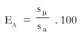
where EA=the statistical efficiency of sampling design A, expressed as a percentage
µ s = the standard error of the appropriate statistic, e.g., mean, produced by an unrestricted single-stage sample of size n
σA = the standard error of the appropriate statistic, produced by sampling design A of size n.
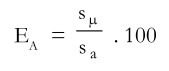
If the degree of precision required is specified in advance, regardless of the sample design, then the relative size of the sample required would indicate efficiency.
Symobolically,
where EA = the efficiency of sampling design A, based on relative sample size and express as a percentage.
It may be noted that when a comparison is made of standard errors of the mean of different sample designs requiring the same rupee expenditure, it will indicate relative economic efficiency. In other words, economic efficiency is measured in terms of the precision of results per rupees of cost. Marketing researchers are generally concerned with economic efficiency of sample designs and aim at obtaining maximum efficiency of this type.
Determining the Size of Non-probability Samples: The preceding discussion was in respect of probability samples. However, non-probability samples are used, perhaps more frequently, in marketing research than probability samples. The question is – How should the size of a non-probability sample be determined? In this case, there is no theoretical basis for estimating sampling error. We have seen how important the concept of sampling error is in determining size when the sample is based on probability.
Generally, two approaches are followed in respect of non-probability samples. One approach is to determine the size as if it were a probability sample. Another approach is to take as large a sample as possible within the constraints of time and money. For example, if a sum of Rs.50,000 has been earmarked for a research project, the estimated fixed costs of sampling and the non-sampling costs are Rs.30,000, and sampling costs are Rs.25 per element, the sample size (n) should be Rs.50,000 – Rs.30,000 / Rs.25 = 800. There are two limitations of this approach. It fails to take into consideration the different in value of information of the sample of 800 as compared to that of other sample sizes. Second, unlike the probability sample, it usually fails to consider trade-offs between sampling and non-sampling errors.
