Conjoint analysis is a statistical technique used in market research to determine how people value different attributes (feature, function, benefits) that make up an individual product or service.
The objective of conjoint analysis is to determine what combination of a limited number of attributes is most influential on respondent choice or decision making. A controlled set of potential products or services is shown to respondents and by analyzing how they make preferences between these products, the implicit valuation of the individual elements making up the product or service can be determined. These implicit valuations (utilities or part-worths) can be used to create market models that estimate market share, revenue and even profitability of new designs.
Conjoint originated in mathematical psychology and was developed by marketing professor Paul Green at the Wharton School of the University of Pennsylvania and Data Chan. Other prominent conjoint analysis pioneers include professor V. “Seenu” Srinivasan of Stanford University who developed a linear programming (LINMAP) procedure for rank ordered data as well as a self-explicated approach, Richard Johnson (founder of Sawtooth Software) who developed the Adaptive Conjoint Analysis technique in the 1980s and Jordan Louviere (University of Iowa) who invented and developed Choice-based approaches to conjoint analysis and related techniques such as MaxDiff.
Today it is used in many of the social sciences and applied sciences including marketing, product management, and operations research. It is used frequently in testing customer acceptance of new product designs, in assessing the appeal of advertisements and in service design. It has been used in product positioning, but there are some who raise problems with this application of conjoint analysis (see disadvantages).
Conjoint analysis techniques may also be referred to as multiattribute compositional modeling, discrete choice modeling, or stated preference research, and is part of a broader set of trade-off analysis tools used for systematic analysis of decisions. These tools include Brand-Price Trade-Off, Simalto, and mathematical approaches such as AHP, evolutionary algorithms or Rule Developing Experimentation.
Conjoint (trade-off) analysis is one of the most widely-used quantitative methods in Marketing Research. It is used to measure preferences for product features, to learn how changes to price affect demand for products or service, and to forecast the likely acceptance of a product if brought to market.
Rather than directly ask survey respondents what they prefer in a product, or what attributes they find most important, conjoint analysis employs the more realistic context of respondents evaluating potential product profiles. Each profile includes multiple conjoined product features
Steps in Developing a Conjoint Analysis
Developing a conjoint analysis involves the following steps
- Choose product attributes, for example, appearance, size, or price.
- Choose the values or options for each attribute. For example, for the attribute of size, one may choose the levels of 5″, 10″, or 20″. The higher the number of options used for each attribute, the more burden that is placed on the respondents.
- Define products as a combination of attribute options. The set of combinations of attributes that will be used will be a subset of the possible universe of products.
- Choose the form in which the combinations of attributes are to be presented to the respondents. Options include verbal presentation, paragraph description, and pictorial presentation.
- Decide how responses will be aggregated. There are three choices – use individual responses, pool all responses into a single utility function, or define segments of respondents who have similar preferences.
- Select the technique to be used to analyze the collected data. The part-worth model is one of the simpler models used to express the utilities of the various attributes. There also are vector (linear) models and ideal-point (quadratic) models.
Example
Suppose we want to market a new golf ball. We know from experience and from talking with golfers that there are three important product features:
- Average Driving Distance
- Average Ball Life
- Price
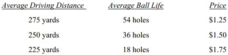
We further know that there is a range of feasible alternatives for each of these features, for instance.
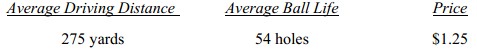
Obviously, the market’s “ideal” ball would be and the “ideal” ball from a cost of manufacturing perspective would be
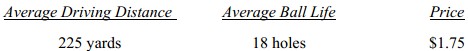
Assuming that it costs less to produce a ball that travels a shorter distance and has a shorter life.
Here’s the basic marketing issue: We’d lose our shirts selling the first ball and the market wouldn’t buy the second. The most viable product is some where in between, but where? Conjoint analysis lets us find out where.
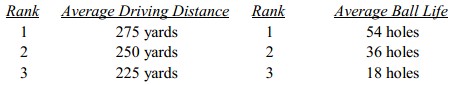
A traditional research project might start by considering the rankings for distance and ball life in below figure
This type of information doesn’t tell us anything that we didn’t already know about which ball to produce. Now consider the same two features taken conjointly. Figures 2a and 2b show the rankings of the 9 possible products for two buyers assuming price is the same for all combinations.
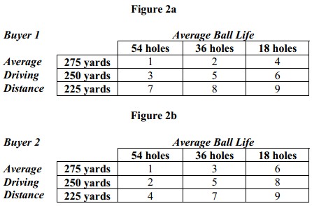
Both buyers agree on the most and least preferred ball. But as we can see from their other choices, Buyer 1 tends to trade-off ball life for distance, whereas Buyer 2 makes the opposite trade-off. The knowledge we gain in going from Figure 1 to Figures 2a and 2b is the essence of conjoint analysis. If you understand this, you understand the power behind this technique.
Next, let’s figure out a set of values for driving distance and a second set for ball life for Buyer 1 so that when we add these values together for each ball they reproduce Buyer 1’s rank orders. Figure 3 shows one possible scheme.

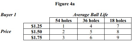
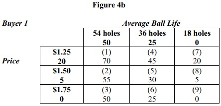
Notice that we could have picked many other sets of numbers that would have worked, so there is some arbitrariness in the magnitudes of these numbers even though their relationships to each other are fixed. Next suppose that Figure 4a represents the trade-offs Buyer 1 is willing to make between ball life and price. Starting with the values we just derived for ball life, Figure 4b shows a set of values for price that when added to those ball life reproduce the rankings for Buyer 1 in Figure 4a.
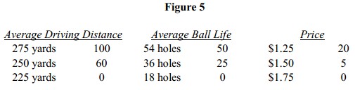
We now have in Figure 5 a complete set of values (referred to as “utilities” or “part-worths”) that capture Buyer 1′ s trade-offs.
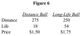
Let’s see how we would use this information to determine which ball to produce. Suppose we were considering one of two golf balls shown in Figure 6.
The values for Buyer 1 in Figure 5 when added together give us an estimate of his preferences. Applying these to the two golf balls we’re considering, we get the results in Figure 7.
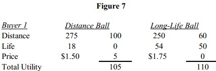
We’d expect buyer 1 to prefer the long-life ball over th e distance ball since it has the larger total value. It’s easy to see how this can be generalized to several different balls and to a representative sample of buyers.
These three steps–collecting trade-offs, estimating buyer value systems, and making choice predictions– form the basics of conjoint analysis. Although trade-off matrices are useful for explaining conjoint analysis as in this example, not many researchers use them nowadays. It’s easier to collect conjoint data by having respondents rank or rate concept statements or by using PC-based interviewing software that decides what questions to ask each respondent, based on his previous answers.
