Having considered the meaning of causation and the types of evidence required to infer causal relationships in the preceding pages, we now turn to some specific designs of causal studies.
Causal inference studies can be divided into two broad categories – natural experiments and controlled experiments. The main point of distinction between the two is the degree of intervention or manipulation exercised by the investigator in a given study. Thus, a natural experiment will involve hardly any intervention of the investigator, except to the extent required for measurement. A controlled experiment, in contrast, will involve his intervention to control and manipulate variables.
Natural Experiments: There are three classes of designs for natural experiments – (i) time-series and trend designs, (ii) cross-sectional designs; and (iii) a combination of the two.
Tim e-series and Trend Designs
In a time-series design, data are obtained from the same sample or population at successive intervals. Generally, current data are obtained from a panel of individuals or households. Other panels such as wholesalers, retail stores or manufactures can also be used. While time-series data relate to the same sample, trend data relate to matched samples drawn from the same population at successive intervals. Thus, there is no continuity in the sample in trend designs, as a result of which data can be analysed in the aggregated form. Since time-series data relate to the same sample over time, change in individual sample units can be analysed. An analysis of this type is also called longitudinal analysis.
There can be several variants of time series and trend designs. At one extreme they need at least one treatment and a subsequent measurement, at the other extreme, they may have several treatments and measurements. A few types of time-series and trend designs are briefly discussed below.
The one-shot case study the design is also known as the ‘try out’ design. It is the simplest and can be shown symbolically as follows:
X O (1)
Where ‘X’ indicates the exposure of a subject or group to an experimental treatment whose effect is to be observed, and ‘O’ indicates the observation or measurement taken on the subject or group after an experimental treatment. Suppose that we provide training to a group of salesmen (X) for a certain period and then measure the sales affected by this group of salesmen (O). Since we do not have a prior measurement of sales made by each of the salesmen trained, it is not possible to measure the effect of training. On account of this major limitation, the design is used only in exploratory research. It should be avoided as far as possible.
Before after without control group: This design differs from the preceding one in one respect, i.e. it has a prior measurement as well. Symbolically, it can be shown as
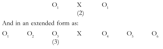
Taking out earlier example, the sales made by salesmen at period (1) are known to us. We now provide them training for a certain period, and then their sales. A comparison of sales after training is made with sales made during the corresponding period before training. Thus the effectiveness of training can be measured by O2-O1. The extended form of the design (3), is an improvement over design (2) as it shows that sales made by a group of salesmen X are measured for three successive periods prior to training and three successive periods after their training.
Although this design is widely used in marketing studies, it fails to provide effective conclusions. For example, there may be several extraneous factors which affect the volume of sales. There may be a lack of competition or a spurt in income which may increase sales at a later period. There are other limitations as well such as the testing effect, which implies that measurement in a subsequent period may be affected by an earlier measurement.
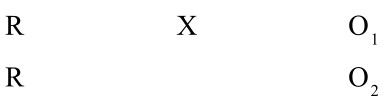
Multiple time-series Another time-series design involves the control group. Symbolically,
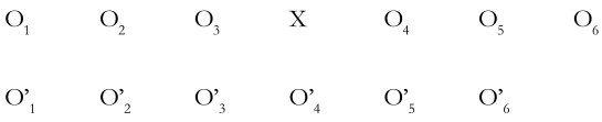
Where the O’s represent measurement of the control group. This design is an improvement over design (3) as it measures the effect of a specific treatment on the experimental group and compares it against the control group. Thus taking our earlier example of training salesmen, two comparable groups of salesmen are selected. Before the treatment i.e. training, sales made by them for three successive time periods are measured for both the groups. Now the experimental group is given training. After the training, sales made by the experimental group as also those made by the control group (which was not given training) are measured. The difference between the average sales for the experimental group and the control group may then be attributed to training.
This design is generally used by selecting panels of individuals or households. Although this design is a substantial improvement over design (3), it suffers from some of the same limitations as were pointed out earlier. Thus, it fails to control history and there may be certain environmental changes in the later period, which may affect effectiveness of the results. Also, results may be altered by the testing effect, i.e. respondents subjected to repeated testing show some peculiar reaction to the experimental stimulus.
Cross-Sectional Designs
In cross-sectional designs, the effect of different levels of treatments is measured on several groups at the same time. Symbolically, a cross-sectional design may be shown as follows:
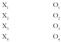
Thus, subscripts 1,2,3,4 show different groups of X given differing treatments. The corresponding measures after the treatments are indicated by O1, O2, O3, and O4. Cross-sectional designs are used when varying levels of advertising is done for the same product but in different territories or when varying prices are fixed in different territories. The impact of varying levels of treatment is studies on the basis of the sales of the product in different territories.
The design also suffers from some of the limitations applicable to earlier designs. Thus, there may be extraneous factors that may affect the sale in a particular territory.
Combination of Cross-sectional and Tim e-series Designs
These designs, as the name implies, combine the time-series and cross-sectional designs. While there can be many variants, a more frequently used design is the ex-post –facto test-control group. The design can be shown symbolically as follows:
Such a design is well suited to continuous panel data. A certain advertisement (X) is run and panel members are then asked if they had seen it earlier. Those who had may constitute a test or experimental group and those who had not form the control group. It may be noted here that the experimental and control groups would not be known until after the advertisement was run. The impact of the advertisement is measured by comparing the difference in purchases made by the experimental and control groups before and after the advertisement.
It will be seen that the experimental and control groups were formed on the basis of whether the panel members had seen the advertisement or not. This self-selection feature of the design may be a source of systematic error. Besides, the testing effect may contribute to inaccuracy. Despite these limitations, this design provides data both cheaply and promptly if the panel already exists.
Controlled Experiments: We have seen in the preceding pages that ‘before-after’ experimental designs without control were subject to certain limitations, i.e. history, maturation, pre-testing and measurement variation. History may cause the ‘before’ and ‘after’ measurements to differ. There may be certain developments during the intervening period as a result of which the two measurements may not be comparable. The second factor is maturation which signifies biological and psychological changes in the subject which take place with the passage of time. For example, the subjects may react very differently ‘before’ a television commercial is shown to them and after the programme. The third factor is the pre-testing which may affect the internal validity of the before-after design. If the consumers are asked about a particular product before the commercial on the television is shown, their responses to the after measurement could be influenced. Finally, variation in measurement may cause variations in the before and after measurements and these may be taken as the effect of the experimental variable. The foregoing limitations indicate the need for a control group against which the results in the experimental group can be compared.
In controlled experiments, two kinds of intervention on the part of the researcher are required. The first relates to the manipulation of at least one assumed independent or causal variable. In other to measure the effect of one or more treatments on the experimental variable, it is necessary that the researcher manipulates at least one variable. The second intervention relates to the assignment of subjects to experimental and control groups on a random basis. This is necessary so that the effect of extraneous factors can be controlled. As the size of the experimental and the control group increases the effect of extraneous factors on these groups on a random basis. This is necessary so that the effect of extraneous factors can be controlled. As the size of the experimental and control group increases, the effect of extraneous factors on these groups can be equalized or balanced by using a random selection procedure. A few experimental designs are as follows:
After-only With Control Group: This is the simplest of all the controlled experimental designs. In this design, only one treatment is given and then both the experimental and the control groups are measure. Symbolically, it can be shown as follows:
It has been criticised on the ground that it does not concern itself with the pre-test. However, by avoiding the pre-test, the design provides control over the testing and instrument effects. This design is particularly suitable in those cases where before measurement or pre-testing is not possible or where testing and instrument effects are likely to be serious.
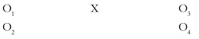
Before –After With One Control Group: This design provides for pre-testing or before measurements. It can be shown symbolically as follows:
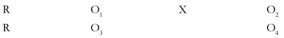
Unlike design (6), this design provides for the selection of the experimental and control groups through the random method. The design is able to control most of the sources of systematic error. Both maturation and the testing effect may be taken as controlled in this design because of their presence in both the experimental and control groups. As the two before measurements, O1 and O3 and the two after measurements, O2 and O4 are made at the same points in time, the design is able to control history.
With the help of this design, one can measure the effect of treatments in three ways: O2 – O1, O2 O4 and (O2 –O1)- (O4- O3). If these measures show similar results, the effect of experimental treatments can be inferred with greater confidence.
Four –Group, Six-study Design: When the investigator has to obtain data from respondents in an undisguised manner, the ‘before-after with control group’ design, such as the preceding one, is not suitable. This is because both the experimental and control groups are likely to be influenced by the before measurement. To overcome this difficulty, a four-group, six-study design may be used. Such a design is extremely suitable in all those cases where some sort of an interaction between the respondent and the questioning process takes place. Symbolically, the design can be shown as follows:
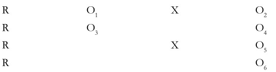
This is a combination of designs(7) and (8). The effect of the treatment can be measured in several ways such as O2-O-1, O4- O2, O6-O5, O4-O3 and (O2-O1)-(O4-O3). The after measurements can be shown in a 2×2 table as follows:
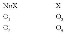
Before measurements taken
No before measurements taken
The difference between ‘No X’ and ‘X’ column means shows the effect of the treatment. Similarly, the difference between the row means indicates the basis for estimating the testing effect. Further, the interaction of testing and treatment can be estimated from the differences in the individual cell means15. Finally, the combined effect of history and maturation maybe estimated by
Our discussion of controlled experimental designs was confined to a single variable.- At this stage, it may be necessary to make some observations on experimental research. It is decidedly better than descriptive research as it enables the researcher to ascertain cause and effect, provided a proper hypothesis is formulated. Experimental research is likely to be more useful to management in decision making and in recent years, it gained popularity which shows that it is a very promising area for researchers. While both laboratory and field experiments are useful in marketing, the latter are generally preferred as they are more helpful to management on account of their being more realistic.
Sources of Experimental Errors
After having described the different types of experiments, we now turn to sources of potential errors in experiments. There are several errors which may distort the accuracy of an experiment. These are briefly described below.
History: History refers to the effect of extraneous variables as a result of an event that is external to an experiment occurring at the same time as the experiment. For example, consider the design O1 X O2 where O1 and O2 represent the sales affected by salesmen in an enterprise in the pre-training period and post-training period, respectively and X represents a sales training programme. This experiment is expected to indicate the effectiveness of the sales training programme by showing higher sales in the post-training period as compared to sales in the pre-training period. If the general business conditions have improved during the training period, when the sales could have risen even without the sales training programme
Maturation: Although maturation is similar to history, it differs from it, as the actual outcome is usually less evident. Maturation refers to a gradual change in the experimental units arising due to the passage of time. In our earlier example of training programme, salesmen have become more matured and more experienced due to the passage of time. As a result, the improvement in sales performance cannot be attributed to the training programme alone. Another example could be of consumer panels. The members of such panels forming test units may change their purchase behaviour during the period when an experiment is on. As the time between O1 and O2 becomes longer, the chance of maturation affects also increases.
Pre-measurement effect: This error is caused on account of the changes in the dependent variable as a result of the effect of the initial measurement. For example, consider the case of respondents who were given a pretreatment questionnaire. After their exposure to the treatment, they were given another questionnaire, an alternative form of the questionnaire completed earlier. They may respond differently merely because they are now familiar with the questionnaire. In such a case, respondents’ familiarity with the earlier questionnaire is likely to influence their responses in the subsequent period.
Interactive testing effect: This error arises on account of change in the independent variable as a result of sensitizing effect of the initial measurement. In other words, the first observation affects the reaction to the treatment. For example, consider the case that respondents have been given a pretreatment questionnaire that asks questions about various brands of hair oil. The pretreatment questionnaire may sensitizer them to the hair oil market and distort the awareness level of new introduction, i.e. the treatment. In such a case, the measurement effect cannot be generalised to non-sensitised persons.
Instrumentation: Instrumentation refers to the changes in the measuring instrument over time. For example, consider the case when the interviewer uses a different format of a questionnaire in O2 as compared to that used in O1. This would case an instrumentation effect. A similar example could be of an interviewer who in his enthusiasm and interest in the survey in O1, explained to the respondents whenever there was any difficulty. But the same interviewer gradually loses his interest in the survey and does not explain properly to the respondents in the post-measurement period-O2. Yet another example could be when sales are measured in terms of revenue and the company has increased the prices of its products in the intervening period.
Selection bias: Selection bias refers to assigning of experimental units in such a way that the groups differ on the dependent variable even before the treatment. Such a situation arises when test units may choose their own groups or when the researcher assigns them to groups on the basis of his judgment. To overcome this bias, it is necessary that test units be assigned to treatment groups on a random basis.
Statistical regression: Statistical regression effect occurs when test units have been selected for exposure to the treatment on the basis of an extreme pretreatment measure. For example, a training programme may be devised only for salesmen whose performance have been very poor. Sales increases in the post-treatment period may then be attributed to the regression effect. This is because random occurrences such as weather, health or luck may contribute to the better performance of salesmen in the subsequent period. Thus the effect of training programme may get distorted on account of this factor.
Mortality: Mortality refers to the loss of one of more test units while the experiment is in progress. It may be emphasised that mortality leads to the differential loss of respondents from the various groups. This means that respondents, who left, say group A are different from those who left group B, thus making the groups incomparable. In case the experiment pertains to only the group, mortality effect occurs when responsiveness of the respondents who have remained in the experiment differs from responsiveness of those who have ceased to be in the experiment.
Criteria of Research Design
Having discussed a number of research, and sources of potential experimental errors, we now turn to the criteria which is good research design should have.
The main criterion of a research design is that it must answer the research questions. To do this, it is necessary that proper hypotheses be formulated otherwise there may be a lack of congruence between the research questions and hypothesis.
The second criterion relates to control of independent variables – both the independent variables of the study as also extraneous independent variables. In order to achieve this, it is necessary to follow the random procedure of selection wherever possible. Thus, subjects should be selected at random, they should be assigned to groups at random and experimental treatments should also be assigned to groups at random.
Research design will be good to the extent that randomisation is followed. It must be used wherever it can be. This will ensure confidence in the results as there will be adequate control over the independent variables. Wherever it is not possible to follow this criterion of randomisation, the intrinsic weakness of the research design must be recognized.
The third criterion is generalisability. To what extent can be generalise the results of the study? It is an extremely difficult question to answer. This criterion does indicate that generalisability is a desirable feature of good research for one would certainly like to apply the results to other situations. This is more true in the case of applied research.
