Reliability modeling is the process of predicting or understanding the reliability of a component or system prior to its implementation. Two types of analysis that are often used to model a complete system availability (including effects from logistics issues like spare part provisioning, transport and manpower) behavior are Fault Tree Analysis and reliability block diagrams. On component level the same type of analysis can be used together with others. The input for the models can come from many sources: Testing, Earlier operational experience field data or data handbooks from the same or mixed industries can be used. In all cases, the data must be used with great caution as predictions are only valid in case the same product in the same context is used. Often predictions are only made to compare alternatives.
Block diagrams are widely used in engineering and science and exist in many different forms. They can also be used to describe the interrelation between the components and to define the system. When used in this fashion, the block diagram is then referred to as a reliability block diagram (RBD). A reliability block diagram is a graphical representation of the components of the system and how they are reliability-wise related (connected). (Note: One can also think of an RBD as a logic diagram for the system based on its characteristics.) It should be noted that this may differ from how the components are physically connected.
After defining the properties of each block in a system, the blocks can then be connected in a reliability-wise manner to create a reliability block diagram for the system. The RBD provides a visual representation of the way the blocks are reliability-wise arranged. This means that a diagram will be created that represents the functioning state (i.e. success or failure) of the system in terms of the functioning states of its components. In other words, this diagram demonstrates the effect of the success or failure of a component on the success or failure of the system. For example, if all components in a system must succeed in order for the system to succeed, the components will be arranged reliability-wise in series. If one of two components must succeed in order for the system to succeed, those two components will be arranged reliability-wise in parallel.
An overall system reliability prediction can be made by looking at the reliabilities of the components that make up the whole system or product. In this chapter, we will examine the methods of performing such calculations. The reliability-wise configuration of components must be determined beforehand. For this reason, we will first look at different component/subsystem configurations, also known as structural properties. Unless explicitly stated, the components will be assumed to be statistically independent.
Component Configurations
In order to construct a reliability block diagram, the reliability-wise configuration of the components must be determined. Consequently, the analysis method used for computing the reliability of a system will also depend on the reliability-wise configuration of the components/subsystems. That configuration can be as simple as units arranged in a pure series or parallel configuration. There can also be systems of combined series/parallel configurations or complex systems that cannot be decomposed into groups of series and parallel configurations. The configuration types considered in this reference include:
- Series configuration.
- Simple parallel configuration.
- Combined (series and parallel) configuration.
- Complex configuration.
- k-out-of-n parallel configuration.
Each of these configurations will be presented, along with analysis methods, in the sections that follow.
Series Systems
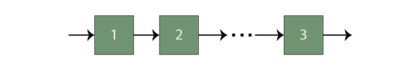
In a series configuration, a failure of any component results in the failure of the entire system. In most cases, when considering complete systems at their basic subsystem level, it is found that these are arranged reliability-wise in a series configuration. For example, a personal computer may consist of four basic subsystems: the motherboard, the hard drive, the power supply and the processor. These are reliability-wise in series and a failure of any of these subsystems will cause a system failure. In other words, all of the units in a series system must succeed for the system to succeed.
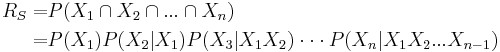
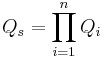
The reliability of the system is the probability that unit 1 succeeds and unit 2 succeeds and all of the other units in the system succeed. So all units must succeed for the system to succeed. The reliability of the system is then given by:
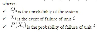
where:
 is the reliability of the system
 is the event of unit being operational
 is probability that unit
  is operational
In the case where the failure of a component affects the failure rates of other components (i.e., the life distribution characteristics of the other components change when one component fails), then the conditional probabilities in equation above must be considered.

However, in the case of independent components, equation above becomes:
or:
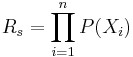
Or, in terms of individual component reliability:
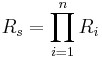
In other words, for a pure series system, the system reliability is equal to the product of the reliabilities of its constituent components.
Example: Calculating Reliability of a Series System
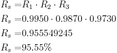
Three subsystems are reliability-wise in series and make up a system. Subsystem 1 has a reliability of 99.5%, subsystem 2 has a reliability of 98.7% and subsystem 3 has a reliability of 97.3% for a mission of 100 hours. What is the overall reliability of the system for a 100-hour mission?
Since the reliabilities of the subsystems are specified for 100 hours, the reliability of the system for a 100-hour mission is simply.
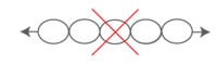
Effect of Component Reliability in a Series System – In a series configuration, the component with the least reliability has the biggest effect on the system’s reliability. There is a saying that a chain is only as strong as its weakest link. This is a good example of the effect of a component in a series system. In a chain, all the rings are in series and if any of the rings break, the system fails. In addition, the weakest link in the chain is the one that will break first. The weakest link dictates the strength of the chain in the same way that the weakest component/subsystem dictates the reliability of a series system. As a result, the reliability of a series system is always less than the reliability of the least reliable component.
Example: Effect of a Component’s Reliability in a Series System
Consider three components arranged reliability-wise in series, where![]()
![]() and
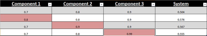
and ![]() (for a given time). In the following table, we can examine the effect of each component’s reliability on the overall system reliability. The first row of the table shows the given reliability for each component and the corresponding system reliability for these values. In the second row, the reliability of Component 1 is increased by a value of 10% while keeping the reliabilities of the other two components constant. Similarly, by increasing the reliabilities of Components 2 and 3 in rows 3 and 4 by a value of 10%, while keeping the reliabilities of the other components at the given values, we can observe the effect of each component’s reliability on the overall system reliability. It is clear that the highest value for the system’s reliability was achieved when the reliability of Component 1, which is the least reliable component, was increased by a value of 10%.
(for a given time). In the following table, we can examine the effect of each component’s reliability on the overall system reliability. The first row of the table shows the given reliability for each component and the corresponding system reliability for these values. In the second row, the reliability of Component 1 is increased by a value of 10% while keeping the reliabilities of the other two components constant. Similarly, by increasing the reliabilities of Components 2 and 3 in rows 3 and 4 by a value of 10%, while keeping the reliabilities of the other components at the given values, we can observe the effect of each component’s reliability on the overall system reliability. It is clear that the highest value for the system’s reliability was achieved when the reliability of Component 1, which is the least reliable component, was increased by a value of 10%.
Table 1: System Reliability for Combinations of Component Reliabilities
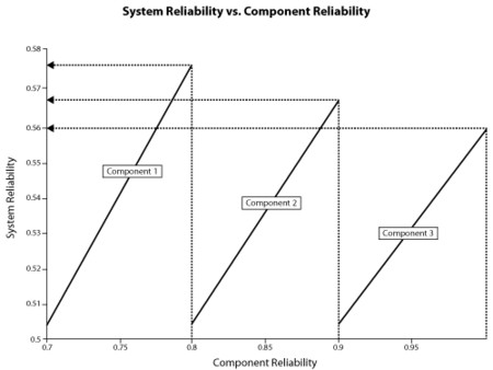
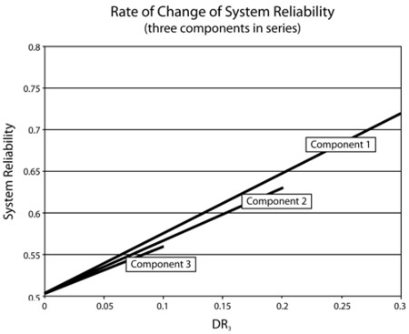
This conclusion can also be illustrated graphically, as shown in the following figure. Note the slight difference in the slopes of the three lines. The difference in these slopes represents the difference in the effect of each of the components on the overall system reliability. In other words, the system reliability’s rate of change with respect to each component’s change in reliability is different. This observation will be explored further when the importance measures of components are considered in later chapters. The rate of change of the system’s reliability with respect to each of the components is also plotted. It can be seen that Component 1 has the steepest slope, which indicates that an increase in the reliability of Component 1 will result in a higher increase in the reliability of the system. In other words, Component 1 has a higher reliability importance.
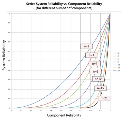
Effect of Number of Components in a Series System – The number of components is another concern in systems with components connected reliability-wise in series. As the number of components connected in series increases, the system’s reliability decreases. The following figure illustrates the effect of the number of components arranged reliability-wise in series on the system’s reliability for different component reliability values. This figure also demonstrates the dramatic effect that the number of components has on the system’s reliability, particularly when the component reliability is low. In other words, in order to achieve a high system reliability, the component reliability must be high also, especially for systems with many components arranged reliability-wise in series.
Example: Effect of the Number of Components in a Series System
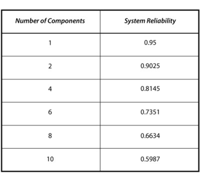
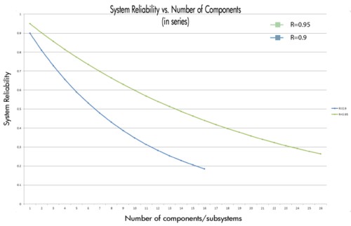
Consider a system that consists of a single component. The reliability of the component is 95%, thus the reliability of the system is 95%. What would the reliability of the system be if there were more than one component (with the same individual reliability) in series? The following table shows the effect on the system’s reliability by adding consecutive components (with the same reliability) in series. The plot illustrates the same concept graphically for components with 90% and 95% reliability.
Simple Parallel Systems
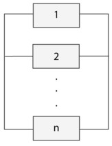
In a simple parallel system, as shown in the figure on the right, at least one of the units must succeed for the system to succeed. Units in parallel are also referred to as redundant units. Redundancy is a very important aspect of system design and reliability in that adding redundancy is one of several methods of improving system reliability. It is widely used in the aerospace industry and generally used in mission critical systems. Other example applications include the RAID computer hard drive systems, brake systems and support cables in bridges.
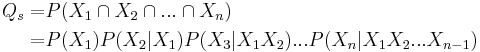
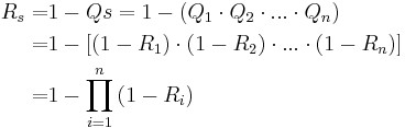
The probability of failure, or unreliability, for a system with n statistically independent parallel components is the probability that unit 1 fails and unit 2 fails and all of the other units in the system fail. So in a parallel system, all n units must fail for the system to fail. Put another way, if unit 1 succeeds or unit 2 succeeds or any of the n units succeeds, then the system succeeds. The unreliability of the system is then given by:
In the case where the failure of a component affects the failure rates of other components, then the conditional probabilities in equation above must be considered. However, in the case of independent components, the equation above becomes:

or:
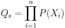
Or, in terms of component unreliability:
Observe the contrast with the series system, in which the system reliability was the product of the component reliabilities; whereas the parallel system has the overall system unreliability as the product of the component unreliabilities. The reliability of the parallel system is then given by:
Example: Calculating the Reliability with Components in Parallel
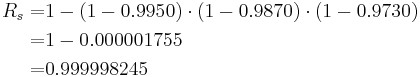
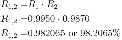
Consider a system consisting of three subsystems arranged reliability-wise in parallel. Subsystem 1 has a reliability of 99.5%, Subsystem 2 has a reliability of 98.7% and Subsystem 3 has a reliability of 97.3% for a mission of 100 hours. What is the overall reliability of the system for a 100-hour mission?
Since the reliabilities of the subsystems are specified for 100 hours, the reliability of the system for a 100-hour mission is:
Combination of Series and Parallel
While many smaller systems can be accurately represented by either a simple series or parallel configuration, there may be larger systems that involve both series and parallel configurations in the overall system. Such systems can be analyzed by calculating the reliabilities for the individual series and parallel sections and then combining them in the appropriate manner. Such a methodology is illustrated in the following example.
Example: Calculating the Reliability for a Combination of Series and Parallel
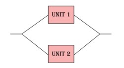
Consider a system with three components. Units 1 and 2 are connected in series and Unit 3 is connected in parallel with the first two, as shown in the next figure.
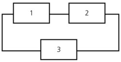
What is the reliability of the system if ![]()
hours? First, the reliability of the series segment consisting of Units 1 and 2 is calculated:
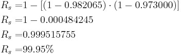
The reliability of the overall system is then calculated by treating Units 1 and 2 as one unit with a reliability of 98.2065% connected in parallel with Unit 3. Therefore:
k-out-of-n Parallel Configuration
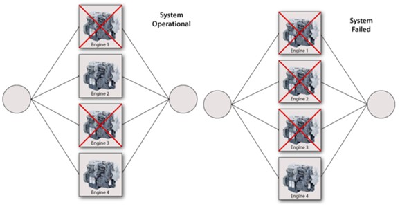
The k-out-of- n configuration is a special case of parallel redundancy. This type of configuration requires that at least components succeed out of the total parallel components for the system to succeed. For example, consider an airplane that has four engines. Furthermore, suppose that the design of the aircraft is such that at least two engines are required to function for the aircraft to remain airborne. This means that the engines are reliability-wise in a k-out-of- n configuration, where k = 2 and n = 4. More specifically, they are in a 2-out-of-4 configuration.
Even though we classified the k-out-of-n configuration as a special case of parallel redundancy, it can also be viewed as a general configuration type. As the number of units required to keep the system functioning approaches the total number of units in the system, the system’s behavior tends towards that of a series system. If the number of units required is equal to the number of units in the system, it is a series system. In other words, a series system of statistically independent components is an n-out-of-n system and a parallel system of statistically independent components is a 1-out-of-n system.
Reliability of k-out-of-n Independent and Identical Components
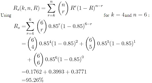
The simplest case of components in a k-out-of-n configuration is when the components are independent and identical. In other words, all the components have the same failure distribution and whenever a failure occurs, the remaining components are not affected. In this case, the reliability of the system with such a configuration can be evaluated using the binomial distribution, or:
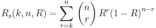
where:
- n is the total number of units in parallel.
- k is the minimum number of units required for system success.
- R is the reliability of each unit.
Example: Calculating the Reliability for a k-out-of-n System
Consider a system of 6 pumps of which at least 4 must function properly for system success. Each pump has an 85% reliability for the mission duration. What i
s the probability of success of the system for the same mission duration?
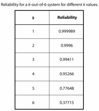
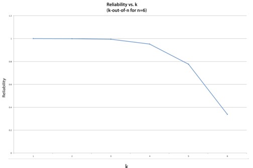
One can examine the effect of increasing the number of units required for system success while the total number of units remains constant (in this example, six units). In the figure above, the reliability of the k-out-of-6 configuration was plotted versus different numbers of required units.
The system configuration becomes a simple parallel configuration for k = 1 and the system is a six-unit series configuration ![]() for
for ![]()
Reliability of Nonidentical k-out-of-n Independent Components – In the case where the k-out-of-n components are not identical, the reliability must be calculated in a different way. One approach, described in detail later in this chapter, is to use the event space method. In this method, all possible operational combinations are considered in order to obtain the system’s reliability. The method is illustrated with the following example.
Example: Calculating Reliability for k-out-of-n , if components are not identical
Three hard drives in a computer system are configured reliability-wise in parallel. At least two of them must function in order for the computer to work properly. Each hard drive is of the same size and speed, but they are made by different manufacturers and have different reliabilities. The reliability of HD #1 is 0.9, HD #2 is 0.88 and HD #3 is 0.85, all at the same mission time.
Since at least two hard drives must be functioning at all times, only one failure is allowed. This is a 2-out-of-3 configuration. The following operational combinations are possible for system success:
- All 3 hard drives operate.
- HD #1 fails while HDs #2 and #3 continue to operate.
- HD #2 fails while HDs #1 and #3 continue to operate.
- HD #3 fails while HDs #1 and #2 continue to operate.
The probability of success for the system (reliability) can now be expressed as:
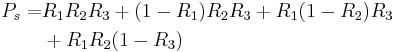
This equation for the reliability of the system can be reduced to:

or:
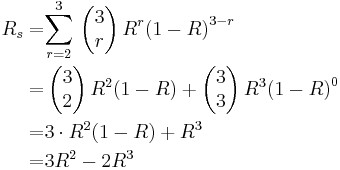
If all three hard drives had the same reliability, R , then the equation for the reliability of the system could be further reduced to:
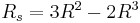
Or, using the binomial approach:
Example 10
Consider the four-engine aircraft discussed previously. If we were to change the problem statement to two out of four engines are required, however no two engines on the same side may fail, then the block diagram would change to the configuration shown below.
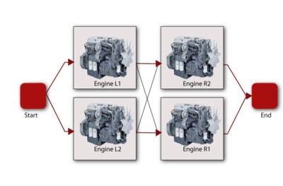
This is the same as having two engines in parallel on each wing and then putting the two wings in series.
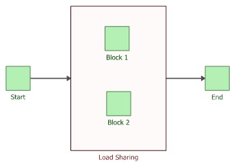
Load Sharing
A reliability block diagram (RBD) allows you to graphically represent how the components within a system are reliability-wise connected. In most cases, independence is assumed across the components within the system. For example, the failure of component A does not affect the failure of component B. However, if a system consists of components that are sharing a load, then the assumption of independence no longer holds true.
If one component fails, then the component(s) that are still operating will have to assume the failed unit’s portion of the load. Therefore, the reliabilities of the surviving unit(s) will change. Calculating the system reliability is no longer an easy proposition. In the case of load sharing components, the change of the failure distributions of the surviving components must be known in order to determine the system’s reliability.
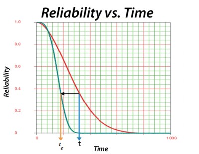
To illustrate this, consider a system of two units connected reliability-wise in parallel as shown below.
Assume that the units must supply an output of 8 volts and that if both units are operational, each unit is to supply 50% of the total output. If one of the units fails, then the surviving unit supplies 100%. Furthermore, assume that having to supply the entire load has a negative impact on the reliability characteristics of the surviving unit.
Because the reliability characteristics of the unit change based on the load it is sharing, a method that can model the effect of the load on life should be used. One way to do this is to use a life distribution along with a life-stress relationship (as discussed in A Brief Introduction to Life-Stress Relationships) for each component. The detailed discussion for this method can be found at Additional Information on Load Sharing. Another simple way is to use the concept of acceleration factors and assume that the load has a linear effect on the failure time. If the load is doubled, then the life of the component will be shortened by half.
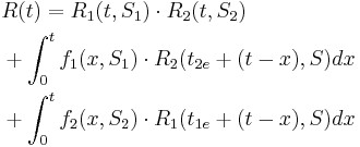
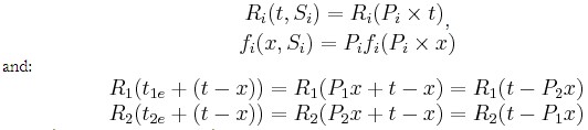
For the above load sharing system, the reliability of each component is a function of time and load. For example, for Unit 1, the reliability and the probability density function are:
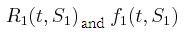
Where, ![]() is the load shared by Unit 1 at time t and the total load of the system is
is the load shared by Unit 1 at time t and the total load of the system is ![]() At the beginning, both units are working. Assume that Unit 1 fails at time x and Unit 2 takes over the entire load. The reliability for Unit 2 at time x is:
At the beginning, both units are working. Assume that Unit 1 fails at time x and Unit 2 takes over the entire load. The reliability for Unit 2 at time x is:
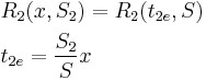
The equivalent time for Unit 2 at time x if it is operated with load S. The equivalent time concept is illustrated in the following plot.
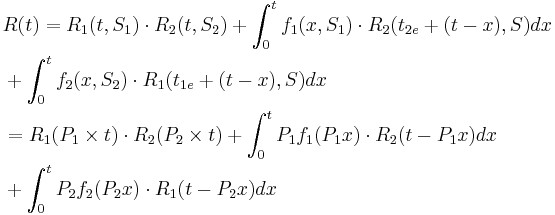
The system reliability at time t is:
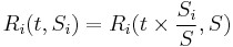
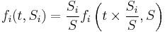
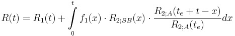
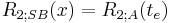
In BlockSim, the failure time distribution for each component is defined at the load of S. The reliability function for a component at a given load is calculated as:
From the above equation, it can be seen that the concept used in the calculation for load sharing is the same as the concept used in the calculation for duty cycle.
Example
In the following load sharing system, Block 1 follows a Weibull failure distribution with
![]() and
and ![]() Block 2 follows a Weibull failure distribution with
Block 2 follows a Weibull failure distribution with ![]() and
and ![]() The load for Block 1 is 1 unit, and for Block 2 it is 3 units. Calculate the system reliability at time 1,500.
The load for Block 1 is 1 unit, and for Block 2 it is 3 units. Calculate the system reliability at time 1,500.
Block 1 shares 25% (P1) of the entire load, and Block 2 shares 75% (P2) of it. Therefore, we have the following equations for calculating the system reliability:
Using the above equations in the system reliability function, we get:
Standby Components
This is a form of redundancy with dependent components. That is, the failure of one component affects the failure of the other(s). This section presents another form of redundancy: standby redundancy. In standby redundancy the redundant components are set to be under a lighter load condition (or no load) while not needed and under the operating load when they are activated.
In standby redundancy the components are set to have two states: an active state and a standby state. Components in standby redundancy have two failure distributions, one for each state. When in the standby state, they have a quiescent (or dormant) failure distribution and when operating, they have an active failure distribution.
In the case that both quiescent and active failure distributions are the same, the units are in a simple parallel configuration (also called a hot standby configuration). When the rate of failure of the standby component is lower in quiescent mode than in active mode, that is called a warm standby configuration. When the rate of failure of the standby component is zero in quiescent mode (i.e., the component cannot fail when in standby), that is called a cold standby configuration.
Simple Standby Configuration
Consider two components in a standby configuration. Component 1 is the active component with a Weibull failure distribution with parameters ![]() and
and ![]() Component 2 is the standby component. When Component 2 is operating, it also has a Weibull failure distribution with
Component 2 is the standby component. When Component 2 is operating, it also has a Weibull failure distribution with ![]() and
and ![]() . Furthermore, assume the following cases for the quiescent distribution.
. Furthermore, assume the following cases for the quiescent distribution.
- Case 1: The quiescent distribution is the same as the active distribution (hot standby).
- Case 2: The quiescent distribution is a Weibull distribution with
 and
and  (warm standby).3
 - Case 3: The component cannot fail in quiescent mode (cold standby).
In this case, the reliability of the system at some time, ![]() , can be obtained using the following equation:
, can be obtained using the following equation:
where:
 is the reliability of the active component.
 is the pdf of the active component.
 is the reliability of the standby component when in standby mode (quiescent reliability).
 is the reliability of the standby component when in active mode.
 is the equivalent operating time for the standby unit if it had been operating at an active mode, such that:
The second equation above can be solved for ![]() and substituted into the first equation above.
and substituted into the first equation above.
