Statistics is the study of the collection, organization, analysis, interpretation and presentation of data. It deals with all aspects of data including the planning of data collection in terms of the design of surveys and experiments.
Terminologies
Various statistics terminologies which are used extensively are
- Data – facts, observations, and information that come from investigations.
- Measurement data sometimes called quantitative data — the result of using some instrument to measure something (e.g., test score, weight);
- Categorical data also referred to as frequency or qualitative data. Things are grouped according to some common property and the number of members of the group are recorded (e.g., males/females, vehicle type).
- Variable – property of an object or event that can take on different values. For example, college major is a variable that takes on values like mathematics, computer science, etc.
- Discrete Variable – a variable with a limited number of values (e.g., gender (male/female).
- Continuous Variable – It is a variable that can take on many different values, in theory, any value between the lowest and highest points on the measurement scale.
- Independent Variable – a variable that is manipulated, measured, or selected by the user as an antecedent condition to an observed behavior. In a hypothesized cause-and-effect relationship, the independent variable is the cause and the dependent variable is the effect.
- Dependent Variable – a variable that is not under the user’s control. It is the variable that is observed and measured in response to the independent variable.
Central Limit Theorem
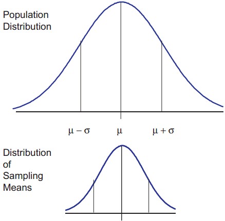
The central limit theorem is the basis of many statistical procedures. The theorem states that for sufficiently large sample sizes ( n ≥ 30), regardless of the shape of the population distribution, if samples of size n are randomly drawn from a population that has a mean µ and a standard deviation σ , the samples’ means X are approximately normally distributed. If the populations are normally distributed, the sample’s means are normally distributed regardless of the sample sizes. Hence, for sufficiently large populations, the normal distribution can be used to analyze samples drawn from populations that are not normally distributed, or whose distribution characteristics are unknown. The theorem states that this distribution of sample means will have the same mean as the original distribution, the variability will be smaller than the original distribution, and it will tend to be normally distributed.
When means are used as estimators to make inferences about a population’s parameters and n ≥ 30, the estimator will be approximately normally distributed in repeated sampling. The mean and standard deviation of that sampling distribution are given as µx = µ and σx = σ/√n. The theorem is applicable for controlled or predictable processes. Most points on the chart tend to be near the average with the curve’s shape is like bell-shaped and the sides tend to be symmetrical. Using ± 3 sigma control limits, the central limit theorem is the basis of the prediction as, if the process has not changed, a sample mean falls outside the control limits an average of only 0.27% of the time. The theorem enables the use of smaller sample averages to evaluate any process because distributions of sample means tend to form a normal distribution.
Descriptive Statistics
Central Tendencies – Central tendency is a measure that characterizes the central value of a collection of data that tends to cluster somewhere between the high and low values in the data. It refers to measurements like mean, median and mode. It is also called measures of center. It involves plotting data in a frequency distribution which shows the general shape of the distribution and gives a general sense of how the numbers are grouped. Several statistics can be used to represent the “center” of the distribution.
- Mean – The mean is the most common measure of central tendency. It is the ratio of the sum of the scores to the number of the scores. For ungrouped data which has not been grouped in intervals, the arithmetic mean is the sum of all the values in that population divided by the number of values in the population as

Where, µ is the arithmetic mean of the population, Xi is the ith value observed, N is the number of items in the observed population and ∑ is the sum of the values. For example, the production of an item for 5 days is 500, 750, 600, 450 and 775 then the arithmetic mean is µ = 500 + 750 + 600 + 450 + 775/ 5 = 615. It gives the distribution’s arithmetic average and provides a reference point for relating all other data points. For grouped data, an approximation is done using the midpoints of the intervals and the frequency of the distribution as

- Median – It divides the distribution into halves; half are above it and half are below it when the data are arranged in numerical order. It is also called as the score at the 50th percentile in the distribution. The median location of N numbers can be found by the formula (N + 1) / 2. When N is an odd number, the formula yields an integer that represents the value in a numerically ordered distribution corresponding to the median location. (For example, in the distribution of numbers (3 1 5 4 9 9 8) the median location is (7 + 1) / 2 = 4. When applied to the ordered distribution (1 3 4 5 8 9 9), the value 5 is the median. If there were only 6 values (1 3 4 5 8 9), the median location is (6 + 1) / 2 = 3.5 hence, median is half-way between the 3rd and 4th scores (4 and 5) or 4.5. It is the distribution’s center point or middle value with an equal number of data points occur on either side of the median but useful when the data set has extreme high or low values and used with non-normal data
- Mode – It is the most frequent or common score in the distribution or the point or value of X that corresponds to the highest point on the distribution. If the highest frequency is shared by more than one value, the distribution is said to be multimodal and with two, it is bimodal or peaks in scoring at two different points in the distribution. For example in the measurements 75, 60, 65, 75, 80, 90, 75, 80, 67, the value 75 appears most frequently, thus it is the mode.
Measures of Spread – Although the average value in a distribution is informative about how scores are centered in the distribution, the mean, median, and mode lack context for interpreting those statistics. Measures of variability provide information about the degree to which individual scores are clustered about or deviate from the average value in a distribution.
- Range – The simplest measure of variability to compute and understand is the range. The range is the difference between the highest and lowest score in a distribution. Although it is easy to compute, it is not often used as the sole measure of variability due to its instability. Because it is based solely on the most extreme scores in the distribution and does not fully reflect the pattern of variation within a distribution, the range is a very limited measure of variability.
- Inter-quartile Range (IQR) – Provides a measure of the spread of the middle 50% of the scores. The IQR is defined as the 75th percentile – the 25th percentile. The inter-quartile range plays an important role in the graphical method known as the box plot. The advantage of using the IQR is that it is easy to compute and extreme scores in the distribution have much less impact but its strength is also a weakness in that it suffers as a measure of variability because it discards too much data. Researchers want to study variability while eliminating scores that are likely to be accidents. The box plot allows for this for this distinction and is an important tool for exploring data.
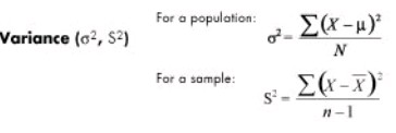
- Variance (σ2) – The variance is a measure based on the deviations of individual scores from the mean. As, simply summing the deviations will result in a value of 0 hence, the variance is based on squared deviations of scores about the mean. When the deviations are squared, the rank order and relative distance of scores in the distribution is preserved while negative values are eliminated. Then to control for the number of subjects in the distribution, the sum of the squared deviations, is divided by N (population) or by N – 1 (sample). The result is the average of the sum of the squared deviations and it is called the variance. The variance is not only a high number but it is also difficult to interpret because it is the square of a value.
- Standard deviation (σ) – The standard deviation is defined as the positive square root of the variance and is a measure of variability expressed in the same units as the data. The standard deviation is very much like a mean or an “average” of these deviations. In a normal (symmetric and mound-shaped) distribution, about two-thirds of the scores fall between +1 and -1 standard deviations from the mean and the standard deviation is approximately 1/4 of the range in small samples (N < 30) and 1/5 to 1/6 of the range in large samples (N > 100).
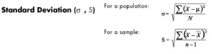
- Coefficient of variation (cv) – Measures of variability can not be compared like the standard deviation of the production of bolts to the availability of parts. If the standard deviation for bolt production is 5 and for availability of parts is 7 for a given time frame, it can not be concluded that the standard deviation of the availability of parts is greater than that of the production of bolts thus, variability is greater with the parts. Hence, a relative measure called the coefficient of variation is used. The coefficient of variation is the ratio of the standard deviation to the mean. It is cv = σ / µ for a population and cv = s/ for a sample.
Measures of Shape – For distributions summarizing data from continuous measurement scales, statistics can be used to describe how the distribution rises and drops.
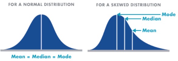
- Symmetric – Distributions that have the same shape on both sides of the center are called symmetric and those with only one peak are referred to as a normal distribution.
- Skewness – It refers to the degree of asymmetry in a distribution. Asymmetry often reflects extreme scores in a distribution. Positively skewed is when it has a tail extending out to the right (larger numbers) so, the mean is greater than the median and the mean is sensitive to each score in the distribution and is subject to large shifts when the sample is small and contains extreme scores. Negatively skewed has an extended tail pointing to the left (smaller numbers) and reflects bunching of numbers in the upper part of the distribution with fewer scores at the lower end of the measurement scale.
Measures of Association – It provides information about the relatedness between variables so as to help estimate the existence of a relationship between variables and it’s strength. They are
- Covariance – It shows how the variable y reacts to a variation of the variable x. Its formula is for a population cov( X, Y ) = ∑( xi − µx) (yi − µy) / N
- Correlation coefficient (r) – It is a number that ranges between −1 and +1. The sign of r will be the same as the sign of the covariance. When r equals−1, then it is a perfect negative relationship between the variations of the x and y thus, increase in x will lead to a proportional decrease in y. Similarly when r equals +1, then it is a positive relationship or the changes in x and the changes in y are in the same direction and in the same proportion. If r is zero, there is no relation between the variations of both. Any other value of r determines the relationship as per how r is close to −1, 0, or +1. The formula for the correlation coefficient for population is ρ = Cov( X, Y ) /σx by
- Coefficient of determination (r2) – It measures the proportion of changes of the dependent variable y as explained by the independent variable x. It is the square of the correlation coefficient r thus, is always positive with values between zero and one. If it is zero, the variations of y are not explained by the variations of x but if it one, the changes in y are explained fully by the changes in x but other values of r are explained according to closeness to zero or one.
Frequency Distributions – A distribution is the amount of potential variation in the outputs of a process, usually expressed by its shape, mean or variance. A frequency distribution graphically summarizes and displays the distribution of a process data set. The shape is visualized against how closely it resembles the bell curve shape or if it is flatter or skewed to the right or left. The frequency distribution’s centrality shows the degree to which the data center on a specific value and the amount of variation in range or variance from the center.
A frequency distribution groups data into certain categories, each category representing a subset of the total range of the data population or sample. Frequency distributions are usually displayed in a histogram. Size is shown on the horizontal axis (x-axis) and the frequency of each size is shown on the vertical axis (y-axis) as a bar graph. The length of the bars is proportional to the relative frequencies of the data falling into each category, and the width is the range of the category. It is used to ascertain information about data like distribution type of the data.
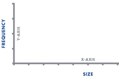
It is developed by segmenting the range of the data into equal sized bars or segments groups then computing and labeling the frequency vertical axis with the number of counts for each bar and labeling the horizontal axis with the range of the response variable. Finally, determining the number of data points that reside within each bar and construct the histogram.
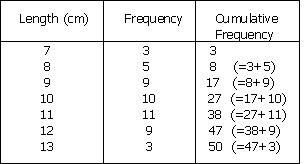
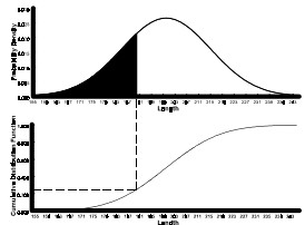
Cumulative Frequency Distribution – It is created from a frequency distribution by adding an additional column to the table called cumulative frequency thus, for each value, the cumulative frequency for that value is the frequency up to and including the frequency for that value. It shows the number of data at or below a particular variable.
The cumulative distribution function, F(x), denotes the area beneath the probability density function to the left of x.
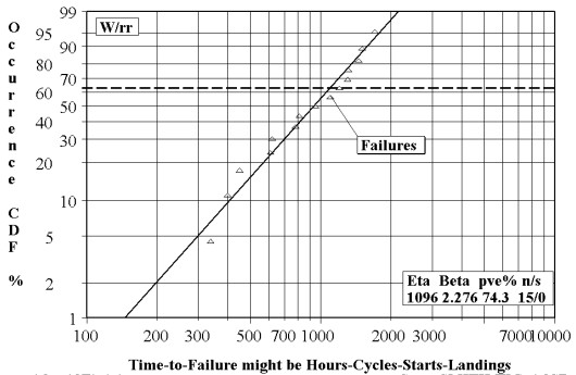
Weibull Plots – It is usually used to estimate the cumulative probability that a given sample will fail under certain conditions. The data can be used to determine a point at which a certain number of samples will fail. Once it is known, this information can help design a process such that no part of the sample approaches the stress limitations. It provides reasonably accurate failure analysis and forecasts with extremely small samples by providing a simple and useful graphical plot of the failure data.
The Weibull plot has special scales designed so that the data points will be almost linear if they follow a Weibull distribution. The Weibull distribution has three parameters but can use only two if the third is assumed
- α is the shape parameter
- θ is the scale parameter
- γ is the location parameter
Weibull plots usually chart data on the probable life of a product or process which is measured in hours, miles, or any other metric that describes the time-to-failure. If complete data is available, the exact time-to-failure is known but for suspended data or right censored, the unit operates successfully for a known period of time and could have continued for an additional period of time that is not known whereas, for interval data or left censored, the time-to failure is known but only within a certain range of time.