In typical life data analysis, the practitioner analyzes life data from a sampling of units operated under normal conditions. This analyses allows the practitioner to quantify the life characteristics of the product and make general predictions about all of the products in the population. For a variety of reasons, engineers may wish to obtain reliability results for their products more quickly than they can with data obtained under normal operating conditions. As an alternative, these engineers may use quantitative accelerated life tests to capture life data under accelerated stress conditions that will cause the products to fail more quickly without introducing unrealistic failure mechanisms.
Accelerated life testing is the process of testing a product by subjecting it to conditions (stress, strain, temperatures, voltage, vibration rate, pressure etc.) in excess of its normal service parameters in an effort to uncover faults and potential modes of failure in a short amount of time. By analyzing the product’s response to such tests, engineers can make predictions about the service life and maintenance intervals of a product.
In polymers, testing may be done at elevated temperatures to produce a result in a shorter amount of time than it could be produced at ambient temperatures. Many mechanical properties of polymers have an Arrhenius type relationship with respect to time and temperature (for example, creep, stress relaxation, and tensile properties). If one conducts short tests at elevated temperatures, that data can be used to extrapolate the behavior of the polymer at room temperature, avoiding the need to do lengthy, and hence expensive tests.
Choosing a physical acceleration model is a lot like choosing a life distribution model. First identify the failure mode and what stresses are relevant (i.e., will accelerate the failure mechanism). Then check to see if the literature contains examples of successful applications of a particular model for this mechanism. Various models to be considered for selection are
- Arrhenius
- The (inverse) power rule for voltage
- The exponential voltage model
- Two temperature/voltage models
- The electromigration model
- Three stress models (temperature, voltage and humidity)
- Eyring (for more than three stresses or when the above models are not satisfactory)
- The Coffin-Manson mechanical crack growth model
All but the last model (the Coffin-Manson) apply to chemical or electronic failure mechanisms, and since temperature is almost always a relevant stress for these mechanisms, the Arrhenius model is nearly always a part of any more general model. The Coffin-Manson model works well for many mechanical fatigue-related mechanisms.
Sometimes models have to be adjusted to include a threshold level for some stresses. In other words, failure might never occur due to a particular mechanism unless a particular stress (temperature, for example) is beyond a threshold value. A model for a temperature-dependent mechanism with a threshold at T=T0 might look like
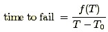
for which f(T) could be Arrhenius. As the temperature decreases towards T0, time to fail increases toward infinity in this (deterministic) acceleration model.
In general, use the simplest model (fewest parameters) you can. When you have chosen a model, use visual tests and formal statistical fit tests to confirm the model is consistent with your data. Continue to use the model as long as it gives results that “work,” but be quick to look for a new model when it is clear the old one is no longer adequate.
Accelerated life testing involves the acceleration of failures with the single purpose of quantifying the life characteristics of the product at normal use conditions. More specifically, accelerated life testing can be divided into two areas: qualitative accelerated testing and quantitative accelerated life testing. In qualitative accelerated testing, the engineer is mostly interested in identifying failures and failure modes without attempting to make any predictions as to the product’s life under normal use conditions. In quantitative accelerated life testing, the engineer is interested in predicting the life of the product (or more specifically, life characteristics such as MTTF, etc.) at normal use conditions, from data obtained in an accelerated life test.
Each type of test that has been called an accelerated test provides different information about the product and its failure mechanisms. These tests can be divided into two types: qualitative tests (HALT, HAST, torture tests, shake and bake tests, etc.) and quantitative accelerated life tests. This reference addresses and quantifies the models and procedures associated with quantitative accelerated life tests (QALT).
Qualitative Accelerated Testing
Qualitative tests are tests which yield failure information (or failure modes) only. They have been referred to by many names including elephant tests, torture tests, HALT, Shake & bake tests.
Qualitative tests are performed on small samples with the specimens subjected to a single severe level of stress, to multiple stresses, or to a time-varying stress (e.g., stress cycling, cold to hot, etc.). If the specimen survives, it passes the test. Otherwise, appropriate actions will be taken to improve the product’s design in order to eliminate the cause(s) of failure. Qualitative tests are used primarily to reveal probable failure modes. However, if not designed properly, they may cause the product to fail due to modes that would never have been encountered in real life. A good qualitative test is one that quickly reveals those failure modes that will occur during the life of the product under normal use conditions. In general, qualitative tests are not designed to yield life data that can be used in subsequent quantitative accelerated life data analysis as described in this reference. In general, qualitative tests do not quantify the life (or reliability) characteristics of the product under normal use conditions, however they provide valuable information as to the types and levels of stresses one may wish to employ during a subsequent quantitative test.
Quantitative Accelerated Life Testing
Quantitative accelerated life testing (QALT), unlike the qualitative testing methods described previously, consists of tests designed to quantify the life characteristics of the product, component or system under normal use conditions, and thereby provide reliability information. Reliability information can include the probability of failure of the product under use conditions, mean life under use conditions, and projected returns and warranty costs. It can also be used to assist in the performance of risk assessments, design comparisons, etc.
Quantitative accelerated life testing can take the form of usage rate acceleration or overstress acceleration. Both accelerated life test methods are described next. Because usage rate acceleration test data can be analyzed with typical life data analysis methods, the overstress acceleration method is the testing method relevant to both ALTA and the remainder of this reference.
Arrhenius
One of the earliest and most successful acceleration models predicts how time-to-fail varies with temperature. This empirically based model is known as the Arrhenius equation. The Arrhenius life-stress model (or relationship) is probably the most common life-stress relationship utilized in accelerated life testing. It has been widely used when the stimulus or acceleration variable (or stress) is thermal (i.e., temperature). It is derived from the Arrhenius reaction rate equation proposed by the Swedish physical chemist Svandte Arrhenius in 1887. It takes the form
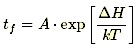
with T denoting temperature measured in degrees Kelvin (273.16 + degrees Celsius) at the point when the failure process takes place and k is Boltzmann’s constant (8.617e-5 in ev/K). The constant A is a scaling factor that drops out when calculating acceleration factors, with ΔH (pronounced “Delta H”) denoting the activation energy, which is the critical parameter in the model.
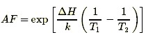
The value of ΔH depends on the failure mechanism and the materials involved, and typically ranges from 0.3 or 0.4 up to 1.5, or even higher. Acceleration factors between two temperatures increase exponentially as ΔH increases. The acceleration factor between a higher temperature T2 and a lower temperature T1 is given by
Using the value of k given above, this can be written in terms of T in degrees Celsius as
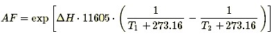
The only unknown parameter in this formula is ΔH.
Example:
The acceleration factor between 25°C and 125°C is 133 if ΔH = 0.5 and 17,597 if ΔH = 1.0.
The Arrhenius model has been used successfully for failure mechanisms that depend on chemical reactions, diffusion processes or migration processes. This covers many of the non-mechanical (or non-material fatigue) failure modes that cause electronic equipment failure.
The Power Law
A power law is a functional relationship between two quantities, where one quantity varies as a power of another. For instance, the number of cities having a certain population size is found to vary as a power of the size of the population. Empirical power-law distributions hold only approximately or over a limited range. The Power Law model is a popular method for analyzing the reliability of complex repairable systems in the field.
In the real world, some systems consist of many components. A failure of one critical component would bring down the whole system. After the component is repaired, the system has been repaired. However, because there are many other components still operating with various ages, the system is not put back into a like new condition after the repair of the single component. The repair of a single component is only enough to get the system operational again, which means the system reliability is almost the same as that before it failed. For example, a car is not as good as new after the replacement of a failed water pump. This kind of repair is called minimal repair. Distribution theory does not apply to the failures of a complex system; the intervals between failures of a complex repairable system do not follow the same distribution. Rather, the sequence of failures at the system levels follows a non-homogeneous Poisson process (NHPP).
When the system is first put into service, its age is 0. Under the NHPP, the first failure is governed by a distribution F(x) with failure rate r(x). Each succeeding failure is governed by the intensity function u(x) of the process. Let t be the age of the system and assume that Δt is very small. The probability that a system of age t fails between t and t + Δt is given by the intensity function u(t)Δt; the failure intensity u(t) for the NHPP has the same functional form as the failure rate governing the first system failure. If the first system failure follows the Weibull distribution, the failure rate is
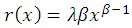
and the system intensity function is:
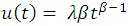
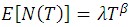
This is the Power Law model. The Weibull distribution governs the first system failure and the Power Law model governs each succeeding system failure. The Power Law mean value function is:
Here T is the system operation end time and N(T) is the number of failures over time 0 to T.

The model is used to subject products to accelerating stresses which are not thermal stress. The model enlists, that the life of the product is inversely proportional to the increased stress.
Example
A device that normally operates with five volts applied is tested at two increased stress levels V1 = 15 volts and V2 = 30 volts.
Five percent of the population failed at 150 hours when the high stress voltage of 30 volts was used. When the stress voltage of 15 volts was applied, five percent of the population failed at 750 hours.
At what time t would five percent of the population be expected to fail under the normal stress of five volts?
[750/150] = [30/15]blog [750/150] = b log [30/15]
b = 2.3
[t /150] = [30/5]2.3t = 9240 hours.
This means that an hour of testing at 30 volts is equivalent to 62 hours of use at five volts.
Properties of power laws
Scale invariance – One attribute of power laws is their scale invariance. Given a relation ![]() , scaling the argument
, scaling the argument ![]() by a constant factor causes only a proportionate scaling of the function itself. That is,
by a constant factor causes only a proportionate scaling of the function itself. That is,

That is, scaling by a constant simply multiplies the original power-law relation by the constant ![]() . Thus, it follows that all power laws with a particular scaling exponent are equivalent up to constant factors, since each is simply a scaled version of the others. This behavior is what produces the linear relationship when logarithms are taken of both
. Thus, it follows that all power laws with a particular scaling exponent are equivalent up to constant factors, since each is simply a scaled version of the others. This behavior is what produces the linear relationship when logarithms are taken of both ![]() and
and ![]() and the straight-line on the log-log plot is often called the signature of a power law. With real data, such straightness is a necessary, but not sufficient, condition for the data following a power-law relation. In fact, there are many ways to generate finite amounts of data that mimic this signature behavior, but, in their asymptotic limit, are not true power laws (e.g., if the generating process of some data follows a Log-normal distribution). Thus, accurately fitting and validating power-law models is an active area of research in statistics.
and the straight-line on the log-log plot is often called the signature of a power law. With real data, such straightness is a necessary, but not sufficient, condition for the data following a power-law relation. In fact, there are many ways to generate finite amounts of data that mimic this signature behavior, but, in their asymptotic limit, are not true power laws (e.g., if the generating process of some data follows a Log-normal distribution). Thus, accurately fitting and validating power-law models is an active area of research in statistics.
No average – Power-laws have a well-defined mean only if the exponent exceeds 2 and have a finite variance only when the exponent exceeds 3; most identified power laws in nature have exponents such that the mean is well-defined but the variance is not, implying they are capable of black swan behavior. This can be seen in the following thought experiment: imagine a room with your friends and estimate the average monthly income in the room. Now imagine the world’s richest person entering the room, with a monthly income of about 1 billion US$. What happens to the average income in the room? Income is distributed according to a power-law known as the Pareto distribution (for example, the net worth of Americans is distributed according to a power law with an exponent of 2).
On the one hand, this makes it incorrect to apply traditional statistics that are based on variance and standard deviation (such as regression analysis). On the other hand, this also allows for cost-efficient interventions. For example, given that car exhaust is distributed according to a power-law among cars (very few cars contribute to most contamination) it would be sufficient to eliminate those very few cars from the road to reduce total exhaust substantially.
Universality – The equivalence of power laws with a particular scaling exponent can have a deeper origin in the dynamical processes that generate the power-law relation. In physics, for example, phase transitions in thermodynamic systems are associated with the emergence of power-law distributions of certain quantities, whose exponents are referred to as the critical exponents of the system. Diverse systems with the same critical exponents—that is, which display identical scaling behaviour as they approach criticality—can be shown, via renormalization group theory, to share the same fundamental dynamics. For instance, the behavior of water and CO2 at their boiling points fall in the same universality class because they have identical critical exponents. In fact, almost all material phase transitions are described by a small set of universality classes. Similar observations have been made, though not as comprehensively, for various self-organized critical systems, where the critical point of the system is an attractor. Formally, this sharing of dynamics is referred to as universality, and systems with precisely the same critical exponents are said to belong to the same universality class.
Power-law functions
Scientific interest in power-law relations stems partly from the ease with which certain general classes of mechanisms generate them. The demonstration of a power-law relation in some data can point to specific kinds of mechanisms that might underlie the natural phenomenon in question, and can indicate a deep connection with other, seemingly unrelated systems. The ubiquity of power-law relations in physics is partly due to dimensional constraints, while in complex systems, power laws are often thought to be signatures of hierarchy or of specific stochastic processes. A few notable examples of power laws are the Gutenberg–Richter law for earthquake sizes, Pareto’s law of income distribution, structural self-similarity of fractals, and scaling laws in biological systems. Research on the origins of power-law relations, and efforts to observe and validate them in the real world, is an active topic of research in many fields of science, including physics, computer science, linguistics, geophysics, neuroscience, sociology, economics and more.
However much of the recent interest in power laws comes from the study of probability distributions: The distributions of a wide variety of quantities seem to follow the power-law form, at least in their upper tail (large events). The behavior of these large events connects these quantities to the study of theory of large deviations (also called extreme value theory), which considers the frequency of extremely rare events like stock market crashes and large natural disasters. It is primarily in the study of statistical distributions that the name “power law” is used; in other areas, such as physics and engineering, a power-law functional form with a single term and a positive integer exponent is typically regarded as a polynomial function.
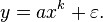
In empirical contexts, an approximation to a power-law![]() often includes a deviation term , ε which can represent uncertainty in the observed values (perhaps measurement or sampling errors) or provide a simple way for observations to deviate from the power-law function (perhaps for stochastic reasons):
often includes a deviation term , ε which can represent uncertainty in the observed values (perhaps measurement or sampling errors) or provide a simple way for observations to deviate from the power-law function (perhaps for stochastic reasons):
Mathematically, a strict power law cannot be a probability distribution, but a distribution that is a truncated power function is possible: ![]() for
for ![]() where the exponent is greater than 1 (otherwise the tail has infinite area), the minimum value is needed otherwise the distribution has infinite area as x approaches 0, and the constant C is a scaling factor to ensure that the total area is 1, as required by a probability distribution. More often one uses an asymptotic power law – one that is only true in the limit; see power-law probability distributions below for details. Typically the exponent falls in the range
where the exponent is greater than 1 (otherwise the tail has infinite area), the minimum value is needed otherwise the distribution has infinite area as x approaches 0, and the constant C is a scaling factor to ensure that the total area is 1, as required by a probability distribution. More often one uses an asymptotic power law – one that is only true in the limit; see power-law probability distributions below for details. Typically the exponent falls in the range ![]() though not always.
though not always.
