Although the average value in a distribution is informative about how scores are centered in the distribution, the mean, median, and mode lack context for interpreting those statistics. Measures of variability provide information about the degree to which individual scores are clustered about or deviate from the average value in a distribution.
- Range – The simplest measure of variability to compute and understand is the range. The range is the difference between the highest and lowest score in a distribution. Although it is easy to compute, it is not often used as the sole measure of variability due to its instability. Because it is based solely on the most extreme scores in the distribution and does not fully reflect the pattern of variation within a distribution, the range is a very limited measure of variability. The whole thing is really based on just two numbers, that highest and lowest value, and this really only gives you a very limited inference that you can make about the data. It is very sensitive to outliers – data points you captured that are well outside the range.
- Inter-quartile Range (IQR) – Provides a measure of the spread of the middle 50% of the scores. The IQR is defined as the 75th percentile – the 25th percentile. The interquartile range plays an important role in the graphical method known as the boxplot. The advantage of using the IQR is that it is easy to compute and extreme scores in the distribution have much less impact but its strength is also a weakness in that it suffers as a measure of variability because it discards too much data. Researchers want to study variability while eliminating scores that are likely to be accidents. The boxplot allows for this for this distinction and is an important tool for exploring data.
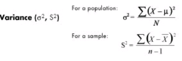
- Variance (σ2) – The variance is a measure based on the deviations of individual scores from the mean. As, simply summing the deviations will result in a value of 0 hence, the variance is based on squared deviations of scores about the mean. When the deviations are squared, the rank order and relative distance of scores in the distribution is preserved while negative values are eliminated. Then to control for the number of subjects in the distribution, the sum of the squared deviations, is divided by N (population) or by N – 1 (sample). The result is the average of the sum of the squared deviations and it is called the variance. The variance is not only a high number but it is also difficult to interpret because it is the square of a value.
It is not expressed in units of data; it’s a measure of the actual variation. For example, if your curve has lots of dispersion and getting to that middle value is important to you, what you’d like to do is make your curve much tighter. The desirable outcome is to come up with a lower level dispersion across the variation of your data. Standard deviation is a measure of dispersion from the mean. Variance is an expression of how much that value is different from the mean, how that’s expressed, and how many sigma values it might stray from that mean over time. There are two types of variance – explained variance measures the proportion of your model and what part of that can be accounted for in the dispersion of the data from a given dataset and unexplained variance breaks that down into two major parts – random variance, which tends to wash out with the aggregation of data, and unidentified or systemic variance, which can definitely introduce bias into your conclusions.
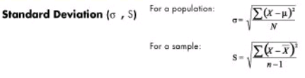
- Standard deviation (σ) – The standard deviation is defined as the positive square root of the variance and is a measure of variability expressed in the same units as the data. The standard deviation is very much like a mean or an “average” of these deviations. In a normal (symmetric and mound-shaped) distribution, about two-thirds of the scores fall between +1 and -1 standard deviations from the mean and the standard deviation is approximately 1/4 of the range in small samples (N < 30) and 1/5 to 1/6 of the range in large samples (N > 100).
In Six Sigma, the empirical rule for standard deviation, is the 68-95-99.7% rule. The empirical rule says that if a population of statistical data has a normal distribution with a population mean and a sensible standard deviation, 68% of the data you’re going to find is going to fall within about one standard deviation from your mean about and 95% of your data is going to be found within two standard deviations from your mean and at about three standard deviations, you’re going to find 99.74% of your data; all the data is going to fall between about three sigmas from a nominal value.
Standard deviation is used only to measure dispersion around the mean and it will always be expressed as a positive value. The reason for that is that it’s a measure of variation. So you express it as a positive value even though on a normal distribution graph you could have -1 sigma or -2 sigma to help show the dispersion around the mean value. Standard deviation is also highly sensitive to outliers. If you have significant outliers way out to the left or way out to the right of three standard deviations, that can give you some real headaches in understanding the data. Having a greater data spread also means that you’ll have a higher standard deviation value.
- Coefficient of variation (cv) – Measures of variability cannot be compared like the standard deviation of the production of bolts to the availability of parts. If the standard deviation for bolt production is 5 and for availability of parts is 7 for a given time frame, it cannot be concluded that the standard deviation of the availability of parts is greater than that of the production of bolts thus, variability is greater with the parts. Hence, a relative measure called the coefficient of variation is used. The coefficient of variation is the ratio of the standard deviation to the mean. It is cv = σ / µ for a population and cv = s/ for a sample.
