Central tendency is a measure that characterizes the central value of a collection of data that tends to cluster somewhere between the high and low values in the data. It refers to measurements like mean, median and mode. It is also called measures of center. It involves plotting data in a frequency distribution which shows the general shape of the distribution and gives a general sense of how the numbers are grouped. Several statistics can be used to represent the “center” of the distribution.
Remember that the central tendency is a distribution of data typically contrasted with this dispersion or variability, so it’s the width of the bell curve that gives you an idea of the amount of dispersion you’re seeing in your data. Then you can use that to judge whether the data has a strong or weak central tendency, based on its dispersion and the general shape of your curve.
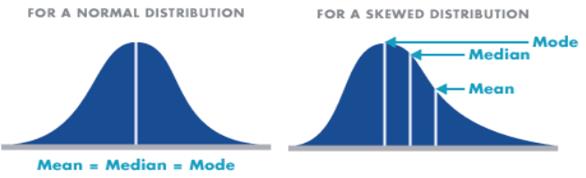
Normal and skewed distribution can be demonstrated through four bell curve examples. The first bell curve graph has the calculated mean or average value in the middle of the curve and has a wide range. The second bell curve has the mean or average value in the middle of the curve and has a narrow range. If you compare the two curves, you can conclude that they both act normally and they have a strong central tendency, but the second curve has a much narrower range of dispersion across the arc than the first one does. They could have exactly the same mean value but a big difference in the range.
- Mean – The mean is the most common measure of central tendency. It is the ratio of the sum of the scores to the number of the scores. For ungrouped data which has not been grouped in intervals, the arithmetic mean is the sum of all the values in that population divided by the number of values in the population as

where, µ is the arithmetic mean of the population, Xi is the ith value observed, N is the number of items in the observed population and ∑ is the sum of the values. For example, the production of an item for 5 days is 500, 750, 600, 450 and 775 then the arithmetic mean is µ = 500 + 750 + 600 + 450 + 775/ 5 = 615. It gives the distribution’s arithmetic average and provides a reference point for relating all other data points. For grouped data, an approximation is done using the midpoints of the intervals and the frequency of the distribution as

- Median – It divides the distribution into halves; half are above it and half are below it when the data are arranged in numerical order. It is also called as the score at the 50th percentile in the distribution. The median location of N numbers can be found by the formula (N + 1) / 2. When N is an odd number, the formula yields an integer that represents the value in a numerically ordered distribution corresponding to the median location. (For example, in the distribution of numbers (3 1 5 4 9 9 8) the median location is (7 + 1) / 2 = 4. When applied to the ordered distribution (1 3 4 5 8 9 9), the value 5 is the median. If there were only 6 values (1 3 4 5 8 9), the median location is (6 + 1) / 2 = 3.5 hence, median is half-way between the 3rd and 4th scores (4 and 5) or 4.5. It is the distribution’s center point or middle value with an equal number of data points occur on either side of the median but useful when the data set has extreme high or low values and used with non-normal data
- Mode – It is the most frequent or common score in the distribution or the point or value of X that corresponds to the highest point on the distribution. If the highest frequency is shared by more than one value, the distribution is said to be multimodal and with two, it is bimodal or peaks in scoring at two different points in the distribution. For example in the measurements 75, 60, 65, 75, 80, 90, 75, 80, 67, the value 75 appears most frequently, thus it is the mode. The mode allows you to get a good handle on what the most commonly occurring value across that entire population is. You need to remember that it’s not necessarily at the center of the dataset. You must also remember that if no value appears more than any other, there really is no mode. You could also find that you can have different conditions around the mode. It could be bimodal, with two modes; trimodal, with three modes; or multimodal. The usefulness of the mode for nominal data is that it can often be seen as the only center value by some experts for analysis purposes. It’s the most frequently found choice. For example, if you’re a retailer, it could be very useful to find out which particular product people buy the most out of a family of products that you’re offering to the market.