EOQ is a mathematical formula designed to minimize the combination of annual holding costs and ordering costs. There is a lot of hype about just in time inventory systems (JIT), which achieve smaller inventories through very frequent orders, but frequent ordering can often result in an over-spending on ordering costs. Even though companies often miscalculate their ordering costs, which make frequent ordering seem costly, EOQ is an important tool for determining what inventory should be
Safety Stock
First of all, here’s the formula so you don’t have to dig through my well-written article for it. Safety Stock: {Z*SQRT (Avg. Lead Time*Standard Deviation of Demand^2 + Avg. Demand^2*Standard Deviation of Lead Time^2}.
Basics of Production Inventory Management
Production inventory management differs from general warehouse management because it involves the determination of how quickly to produce a particular product. The factors involved in many cases are similar, though there are some variances in making the final decision as to how quickly manufacturing should push items through the production line.
Available Materials
Of course, the first concern in production inventory management is on the front end of the process. If you don’t have the materials required for production, then you can’t move forward in providing the products to others. You must make certain that you have all the supplies you need, from raw materials to factory workers, to complete the production process.
Supply and Demand
You must determine the current demand for the product on the market. Good production inventory management occurs when you produce just enough material to satisfy customers’ needs without overextending the production line and manufacturing too many of any given product
You don’t want an incredible amount of back stock lying around, as this detracts from your net profit. On the other hand, you don’t want to be in short supply when a large order comes in, so having a little extra on hand is a great idea, and making sure you are prepared to make a production run for such orders is vital.
Quality Control
Never simply assume that everything manufactured will be flawless. An important consideration in production inventory management is to allow room for error. In other words, calculate a sufficient
Amount of product to assume that, even with flaws that get past quality control efforts, there is sufficient stock of the product required.
Cost Analysis
In many instances, even the best production inventory management strategies fail in the long run due to the cost of the production process being overlooked as a factor. It is important to maintain a cost effective production process, and this includes making sure that your inventory is not an overwhelming factor. This comes back to not MR Producing any items that come off the assembly lines. Doing so is a waste of time and materials, costing you excess money to create.
Obviously, conservation of the materials, time, and energy consumed in manufacturing unnecessary goods is essential to maintaining a cost effective production inventory management strategy. Be proactive in keeping close watch on all occurrences in your production or manufacturing facility to make sure that there is no waste, and you are guaranteed to achieve a greater standard of success and profitability.
Inventory Classifications:
Inventory is idle resources that have future economic value. It indicates that it may be available in different forms depending upon the production cycle stage it is in. Classification of inventory is done on this basis and thus the different classifications of inventory are as follows:
Raw materials – Raw materials are input goods intended for combination and/or conversion through the manufacturing process into semi-finished or finished goods. They change their form and become part of the finished product.
Components and Parts – Just as raw materials are converted to finished goods in a manufacturing operation, components and parts are assembled into finished goods in an assembly operation. Maintenance, repair and operating inventories (MRO) – These include parts, supplies, and materials used in or consumed by routine maintenance and repair of operating equipment, or in support of operations.
In-process goods – These are goods in the process of manufacturing and only partially completed. They are usually measured for accounting purposes in between significant conversion phases. In-process inventories provide the flexibility necessary to deal with variations in demand between different phases of manufacturing.
Finished goods – These represent the completed conversion of raw materials into the final product.
They are goods ready for sale and shipment.
Resale goods – These are goods acquired for resale. Such goods may be purchased by a wholesaler for resale to distributors, or by distributors for resale to consumers, etc.
Capital goods – These are items (such as equipment) that are not used up or consumed during a single. Operating period, but have extended useful lives and must be expensed over multiple operating periods. Tax laws require that such an item be capitalized, and a predetermined percentage of its cost be recognized as an expense each operating period, over a predetermined time frame, according to equipment classes.
Construction materials – These are raw materials and components for construction projects such as a building, bridge, etc.
Hard goods/soft goods – What one identifies as hard goods and soft goods will vary depending on the industry involved. For example, in data processing, hard goods include apparatus such as computers and terminals, while soft goods include software, data storage media, and the like.
Inventory control is concerned with minimizing the total cost of inventory. In the U.K. the term often used is stock control. The three main factors in inventory control decision making process are:
The cost of holding the stock (e.g., based on the interest rate).
The cost of placing an order (e.g., for row material stocks) or the set-up cost of production. The cost of shortage, i.e., what is lost if the stock is insufficient to meet all demand. The third element is the most difficult to measure and is often handled by establishing a “service level” policy, e. g, certain percentage of demand will be met from stock without delay.
The ABC Classification: The ABC classification system is to grouping items according to annual sales volume, in an attempt to identify the small number of items that will account for most of the sales volume and that are the most important ones to control for effective inventory management.
Reorder Point: The inventory level R in which an order is placed where R = D.L, D = demand rate (demand rate period (day, week, etc), and L = lead time.
Safety Stock: Remaining inventory between the times that an order is placed and when new stock is received. If there are not enough inventories then a shortage may occur.
Safety stock is a hedge against running out of inventory. It is an extra inventory to take care on unexpected events. It is often called buffer stock. The absence of inventory is called a shortage.
Quantity Discount Model Calculation Steps:
- Compute EOQ for each quantity discount price.
- Is computed EOQ in the discount range
- If not, use lowest cost quantity in the discount range.
- Compute Total Cost for EOQ or lowest cost quantity in discount range.
- Select quantity with the lowest Total Cost, including the cost of the items purchased.
- The following This JavaScript compute the optimal values for the decision variables based on currently available information about the above factors.
Enter the needed information, and then click the Calculate button.
In entering your data to move from cell to cell in the data-matrix use the Tab key not arrow or enter keys.
MENU:
- The Classical Model
- Shortage Permitted Model
- Production & Consumption Model
- Production & Consumption with Shortage Model
- EOQ with shortage & lead Model
- The ABC Classification
- Inventory Control & uncertain Demand
Inventory System valuation, terminology
Inventory Control Systems: Inventory control is concerned with minimizing the total cost of inventory. The three main factors in inventory control decision making process are:
- The cost of holding the stock (e.g., based on the interest rate).
- The cost of placing an order (e.g., for row material stocks) or the set-up cost of production.
- The cost of shortage, i.e., what is lost if the stock is insufficient to meet all demand.
The third element is the most difficult to measure and is often handled by establishing a “service level” policy, e. g, certain percentage of demand will be met from stock without delay.
In designing an inventory control system, we really provide answers to the three questions:
How often should the inventory status be determined?
This is an internal check system to ascertain that timely action is being taken to replenish the stock
When should a replenishment order be placed?
This shows the actual action to be taken to replenish the stock.
How large should the replenishment order be?
A replenishment order should have a rational about its size. The real problem is to determine the inventory level at which money invested in inventory produces a higher rate of return than it would were it invested in some other phase of the business.
Designing Inventory control systems:
The Demand pattern (D) happens to be the soul of any Inventory control mechanism. Basically inventory control is an attempt to balance the consumption and replenishment of stock of an item in an optimum manner. Obviously, the Demand pattern (D) sets the tone for devising any control measure and therefore while designing inventory control systems the nature of demand pattern viz. independent or dependent needs to be determined first. The Control approaches differ on this differentiation.
Inventory control systems under Independent demand scenario:
Also called the Order-point control systems, Independent demand patterns for an item occur when future demand for it is not related to and is unaffected by its previous demand.
For example, in case of maintenance, repair, and operating supplies, a given item X may be used by many operating departments, and demand by each department may depend on many factors over which there can’t be any control. Therefore, overall demand rates for the item X may vary unpredictably from period to period. In such cases, inventory levels may include provision for safety stock, in addition to the average demand rate, in order to prevent stock-out situation.
For inventories exhibiting independent demand pattern control is exercised based on predetermined order points. Such systems are so designed that whenever a predetermined point in inventory level or in time is reached action to re-order is taken.
There are two basic systems of managing or controlling Inventory under the independent demand pattern:
- Cyclical ordering or Fixed period system (Time Based)
- Order point or fixed order quantity system
Cyclical ordering or fixed period system (Time Based):
Fixed Period based systems (also called “cyclical systems”) are designed so that each inventory item is reviewed and reorders are placed after a predetermined time interval (i.e. every 2 weeks, every 30 days, etc.).
Orders are placed for each item equal to the difference between current inventory level and a predetermined maximum. In cyclical systems, time between reorders is constant, but reorder quantity is variable.
Predetermined maximums are set with a consideration of order lead time. It involves scheduled periodic reviews of the Stock level of all inventory items as follows:
Fixed Schedules (calendar) for reviewing a group of items is drawn
Fixed Desired inventory level (DIL) of each item or group of items is calculated. In case stock level of an item is insufficient to sustain the production operation until the next scheduled review , order is placed to replenish the stock to DIL
Maintenance of perpetual inventory records
Procedure : First , all the inventory items are grouped in certain feasible categories or classes of items such as Pipes & Pipe fittings, Raw materials, Chemicals & Reagents, Oil and Lubricants etc.
Now, a calendar is drawn for all the classes so that depending upon the number of classes each class is reviewed for replenishment during certain specified time frame.
Besides, the DIL or MaxL for each group or individual item is fixed.
Depending upon the Review period, a class of items is reviewed w.e.f. its Stock position, Production plan, any dues in quantity against any previous order.
The DIL or MaxL= (RP+LT+SS) X D
During review and based on the Lead time , if the present stock of an item or group of items is not expected to last the next production plan then action for replenishment is taken by raising the material procurement requisition.
The Order quantity is decided by (MaxL- (Present stock + dues in)
Suitability of the system:
- For materials whose purchases can be planned months in advance
- For materials which exhibit an irregular or seasonal usage pattern
- For items with volatile prices
- For group of items purchased from and shipped together by one supplier
Disadvantages of the system:
- Compels periodic reviews of all items
- Not effective to combat stock out situations
- Actual ordering quantities may deviate from optimum quantity
- Tends to peak the purchasing work load around the review dates
There is no automatic trigger for reorder before the review time in the event of increased usage, which generally leads to increased inventory levels as a means of stock out prevention
System does not permit effective use of economic order quantities
Order point or fixed order quantity system:
Order point system / Fixed Order quantity system of inventory control is based on the (Re)Order point and Order quantity factors rather than on the time factor. The inventory policy, in this system, is drawn, defining the following
- Fixed Order point / Re-Order Level (ROL) for each item
- Fixed Maximum, Minimum levels for each item
- Fixed Quantity to be ordered
Often called Min-Max systems, these involve both a maximum inventory level and a minimum at which reorders are generated. Basically, units of an item are issued until the level of that inventory reaches the predefined reorder point. An order is then triggered for a predetermined quantity (usually a calculated economic order quantity). In this system, the order quantity is constant and the time between orders s variable.
The different Inventory points (Levels) of stock for an item are :
Maximum level (Max.) , predetermined
Minimum Level (Safety stock, SS), predetermined
Lead time (LT) , predetermined
Monthly demand = D (often based on Moving average method)
MaxL.= (Review period + LT + SS) X D
Reorder level (ROL) = (LT + SS) X D
Order Quantity (OQ) = Max. – (Present stock + Pipeline dues)
Process: In course of consumption of an Inventory item, say, in the form of issue from Stores to the users, the stock level of the item starts depleting through its usage rate D.
As per the above definition, the stock goes up to the maximum level in the first replenishment and then, because of steady consumption, comes gradually down. In that process ,again as per the definition , it touches the ROL. As soon as the stock level touches the ROL fresh replenishment action is initiated.
It is presumed that the next lot shall arrive by the time the present depleting stock touches the Safety stock , keeping a stable Lead time and a stable usage rate D.
In some places the Order quantity is decided by the above formula whereas in some other places it is determined by the Economic Order Quantity (EOQ) concept. That’s whenever an order is to be placed the quantity shall be EOQ.
Advantages
Each item is procured in the most economical quantity An item is attended to only when it needs attention i.e. when its stock has reached the ROL Control can be exercised on Inventory w.e.f.. Max & Min levels
Applicability of Order Point system
Item must have a reasonable stable usage
Lead time should not have radical variation
Supplier should be able to accept irregularly timed and unscheduled orders
Limitations of the system
Needs continuous monitoring of stock level of each item Cumbersome to operate for items with unstable usage and lead time perpetual inventory records are required.
Inventory control systems under Dependent demand scenario:
Dependent demand occurs when the need for parts, supplies, or materials is dependent upon a predetermined usage or production schedule.
In such cases, a description and quantity of components needed and the exact date of each need is defined by a production schedule
Required delivery dates for each component will then be offset by lead time, and orders will be placed accordingly. For example, if a pen manufacturing company plans to produce 1000 nos. of a given pen model in a period, it will need 1000 nibs, 1000 caps, etc., and will need them at the rate they will be installed in the finished pens.
Such needs, with consideration for lead time, are considered in a dependent demand planned order schedule.
Material Requirement Planning is one example of a system specifically designed to manage dependent demand reorders.
Role of EQO Basic Inventory Models (Economic Order Quantity / EOQ Models) Economic Order Quantity (EOQ) models are the most basic models of inventory management. The approach in EOW models is essentially to trade-off various relevant costs and derives an order quantity and time for placing an order such, that the total costs are minimized. This note discusses the basic
EOQ model and the sensitivity of costs in EOQ model to various parameters. Later an extension of basic EOQ model is discussed in which case back-orders or shortage are allowed.
Functions of inventory
Though inventory is an idle resource, it is almost essential to keep some inventory in order to promote smooth and efficient running of business.
Consider the case – an enterprise that does not have any inventory. Clearly, as soon as the enterprise receives a sales order, it will have to order for raw materials to complete the order. This will keep the customers waiting. It is quite possible that sales may be lost. Also the enterprise may have to pay high price for some other reasons. On the other hand, inventory may promote sales by reducing customers waiting time. It is essential to maintain the inventories in order to enhance stability of production and employment levels. Consider the case of seasonal items. Any fluctuation in demand can be met if possible, by either changing that part of production or with inventories. However, if the fluctuation is not by changing the rate of production, one has to take into account the following cost.
Cost of increasing production and employment
- Employment and training
- Additional staff and service activities
- Added shifts
- Overtime costs
Cost of decreasing production and employment
- Employee compensation
- other employee costs
- Staff, clerical and service activities
- Total time costs
In other words, the use of seasonal inventories can often after balance of these costs. Broadly, some other functions of inventories are to:
- protect against unpredictable variations (fluctuations) in demand and supply
- take the advantage of price discounts by bulk purchases
- take the advantage of batches and longer production run.
- Provide flexibility to allow changes in production plans in view of change in demands, etc. and
- facilitate intermittent production.
Elementary Inventory Models (with Deterministic Demand)
Let us consider the inventory models in which demand is assumed to be fixed and completely pre-determined.
Notations
D – Annual demand rate
V – Unit purchase cost or unit cost of production (Rs./unit)
A – Ordering or set up cost (Rs/order)
R – Holding cost per Rs. per year (*Rs./Rs/year) (Inventory carrying charges factor)
B – Shortage cost per Rs. short unit time (Rs/ Rs/ year)
Q – Order quantity (to be determined
Inventory Cost
The heart of inventory analysis resides in the identification of relevant costs. Some of the important costs that apply to inventory situation are:
Ordering or set up costs
These are costs associated with ordering or manufacturing goods through purchasing or manufacturing and are known as set up costs or cost of ordering. Set up costs are generally assumed to be independent of the quantity ordered or produced.
Purchase cost or production cost
When large production runs are in process, these results in reduction of production cost per unit. Often, discounts are offered for the purchase of large quantities. In other words, often the unit cost of an item depends on the quantity procured or produced.
Inventory Holding Cost
The cost associated with carrying or holding the goods in stock are known as carrying or holding costs. These costs arise due to the storage costs, property taxes on the items in inventory, interest on the invested capital (interest on value of the inventory items, spillage of the inventory items, depreciation of the inventory items, transportation and handling of the items in inventory, etc.
Shortage or stock out costs
The costs that are incurred as a result of running out of stock are known as stock PUT TO SHORTAGE COSTS. As a result of shortages, sales or goodwill may be lost. If the unfulfilled demand for the items can be satisfied at a later date (back order case), in this case cost of back orders are assumed to vary directly with the shortage quantity (in rupee value) and the delaying time (Rs./ Rs.) . However, if the unfulfilled demand is lost (lost-sales case), in this case cost of shortages are assumed to vary directly with the shortage quantity (Rs./ unit shortage).
Role of EQO Basic Inventory Models
Economic Lot size or Economic Order Quantity Model
Assumptions:
- The rate of demand for the item is deterministic and is constant D units per annum, independent of time.
- Production rate is infinite, i.e. production is instantaneous
- Shortages are not allowed
- Lead time is zero or constant independent of demand and the quantity ordered.
- The entire quantity is delivered as a single package (or production in a single run).
Objective:
To minimize the average annual variable cost.
Problem:
To determine when an order should be placed and how much quantity should be ordered.
The annual variable costs for this problem are two types –
- ordering or set-up cost and
- Inventory holding cost.
As Q is the order quantity and D is the annual demand, the number of orders per years will be D/Q. Therefore, the annual ordering cost will be = A.D/Q …….. (1)
Properties of EOQ model and Sensitivity Analysis
In the above nodal, various parameters are used such as demand (D), inventory carrying charges factor ®, ordering or set-up cost (A). These parameters are estimated and though they are assumed to be known, in real life what we have is an estimated value which may be different than real value for various reasons.
For this reason it is important for practical purposes to test the results of the EQQ model and find how sensitive the results are to the changes in various parameters.
The sensitivity can be explored in various ways. Let the “true” rate of demand is D, “ true” value of order cost is A, “ true” value of inventory holding cost is r and “true” value 9of unit purchase cost or production cost is v. Then the “true” optimal value of order quantity (Q*) will be,
In case when shortage costs are infinitely high (i.e. when shortages are not allowed) b = ¥ and eqn. 17 will reduce to

This is same as equation (6), i.e. optimal order quantity for the E0-model. This is obvious since the EOQ model assume that no shortages are allowed which imply that the shortage are infinite the basic inventory models are given below for easy understanding of the concept as well as to enable one solve the day to day Inventory problems too as far as determining the Economic Order Quantities, Time for ordering etc, .are concerned
The Classical Model
Corporate goals and strategies may sometimes conflict with EOQ. Measuring performance solely by inventory turns is one of the most prolific mistakes made in the name of inventory management. Many companies have achieved aggressive goals in increasing inventory turns only to find their bottom line has shrunk due to increased operational costs.
EOQ is essentially an accounting formula that determines the point at which the combination of order costs and inventory carrying costs are the least. The result is the most cost effective quantity to order. In purchasing this is known as the order quantity, in manufacturing it is known as the production lot size.
While EOQ may not apply to every inventory situation, most organizations will find it beneficial in at least some aspect of their operation. Anytime you have repetitive purchasing or planning of an item, EOQ should be considered. Obvious applications for EOQ are purchase-to-stock distributors and make-to-stock manufacturers, however, make-to-order manufacturers should also consider EOQ when they have multiple orders or release dates for the same items and when planning components and sub-assemblies. Repetitive buy maintenance, repair, and operating (MRO) inventory is also a good application for EOQ. Though EOQ is generally recommended in operations where demand is relatively steady, items with demand variability such as seasonality can still use the model by going to shorter time periods for the EOQ calculation. Just make sure your usage and carrying costs are based on the same time period.
Doesn’t EOQ conflict with Just-In-Time While I don’t want to get into a long discussion on the misconceptions of what Just-In-Time (JIT) is, I will address the most common misunderstanding in which JIT is assumed to mean all components should arrive in the exact run quantities “just in time” for the production run. JIT is actually a quality initiative with the goal of eliminating wasted steps, wasted labor, and wasted cost. EOQ should be one of the tools used to achieve this. EOQ is used to determine which components fit into this JIT model and what level of JIT is economically advantageous for your operation. As an example, let us assume you are a lawn equipment manufacturer and you produce 100 units per day of a specific model of lawn mower. While it may be cost effective to have 100 engines arrive on your dock each day, it would certainly not be cost effective to have 500 screws (1 days supply) used to mount a plastic housing on the lawn mower shipped to you daily. To determine the most cost effective quantities of screws or other components you will need to use the EOQ formula.
The basic Economic Order Quantity (EOQ) formula is as follows:
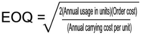
The Inputs
While the calculation itself is fairly simple the task of determining the correct data inputs to accurately represent your inventory and operation is a bit of a project. Exaggerated order costs and carrying costs are common mistakes made in EOQ calculations. Using all costs associated with your purchasing and receiving departments to calculate order cost or using all costs associated with storage and material handling to calculate carrying cost will give you highly inflated costs resulting in inaccurate results from your EOQ calculation. I also caution against using benchmarks or published industry standards in calculations. I have frequently seen references to average purchase order costs of $100 to $150 in magazine articles and product brochures. Often these references trace back to studies performed by advocacy agencies working for business that directly benefit from these exaggerated (my opinion) costs used in ROI calculations for their products or services. I am not denying that some operations may have purchase costs in this range, especially if you are frequently re-sourcing, re-quoting, and/or buying from overseas vendors. However if your operation is primarily involved with repetitive buying from domestic vendors — which is more common — you’ll likely see your purchase order costs in the substantially lower $10 to $30 range.
As you prepare to undertake this project keep in mind that even though accuracy is crucial, small variances in the data inputs generally have very little effect on the outputs. The following breaks down the data inputs in more detail and gives insight into the aspects of each.
Expressed in units, this is generally the easiest part of the equation. You simply input your forecasted annual usage.
Order Cost.
Also known as purchase cost or set up cost, this is the sum of the fixed costs that are incurred each time an item is ordered. These costs are not associated with the quantity ordered but primarily with physical activities required to process the order.
For purchased items, these would include the cost to enter the purchase order and/or requisition, any approval steps, the cost to process the receipt, incoming inspection, invoice processing and vendor payment, and in some cases a portion of the inbound freight may also be included in order cost. It is important to understand that these are costs associated with the frequency of the orders and not the quantities ordered. For example, in your receiving department the time spent checking in the receipt, entering the receipt, and doing any other related paperwork would be included, while the time spent repacking materials, unloading trucks, and delivery to other departments would likely not be included. If you have inbound quality inspection where you inspect a percentage of the quantity received you would include the time to get the specs and process the paperwork and not include time spent actually inspecting, however if you inspect a fixed quantity per receipt you would then include the entire time including inspecting, repacking, etc. In the purchasing department you would include all time associated with creating the purchase order, approval steps, contacting the vendor, expediting, and reviewing order reports, you would not include time spent reviewing forecasts, sourcing, getting quotes (unless you get quotes each time you order), and setting up new items. All time spent dealing with vendor invoices would be included in order cost.
Associating actual costs to the activities associated with order cost is where many an EOQ formula runs afoul. Do not make a list of all of the activities and then ask the people performing the activities “how long does it take you to do this?” The results of this type of measurement are rarely even close to accurate. I have found it to be more effective to determine the percentage of time within the department consumed performing the specific activities and multiplying this by the total labor costs for a certain time period (usually a month) and then dividing by the line items processed during that same period.
It is extremely difficult to associate inbound freight costs with order costs in an automated EOQ program and I suggest it only if the inbound freight cost has a significant effect on unit cost and its effect on unit cost varies significantly based upon the order quantity.
In manufacturing, the order cost would include the time to initiate the work order, time associated with picking and issuing components excluding time associated with counting and handling specific quantities, all production scheduling time, machine set up time, and inspection time. Production scrap directly associated with the machine setup should also be included in order cost as would be any tooling that is discarded after each production run. There may be times when you want to artificially inflate or deflate set-up costs. If you lack the capacity to meet the production schedule using the EOQ, you may want to artificially increase set-up costs to increase lot sizes and reduce overall set up time. If you have excess capacity you may want to artificially decrease set up costs, this will increase overall set up time and reduce inventory investment. The idea being that if you are paying for the labor and machine overhead anyway it would make sense to take advantage of the savings in reduced inventories.
For the most part, order cost is primarily the labor associated with processing the order, however, you can include the other costs such as the costs of phone calls, faxes, postage, envelopes, etc.
Carrying cost
Also called Holding cost, carrying cost is the cost associated with having inventory on hand. It is primarily made up of the costs associated with the inventory investment and storage cost. For the purpose of the EOQ calculation, if the cost does not change based upon the quantity of inventory on hand it should not be included in carrying cost. In the EOQ formula, carrying cost is represented as the annual cost per average on hand inventory unit. Below are the primary components of carrying cost.
Interest: If you had to borrow money to pay for your inventory, the interest rate would be part of the carrying cost. If you did not borrow on the inventory, but have loans on other capital items, you can use the interest rate on those loans since a reduction in inventory would free up money that could be used to pay these loans. If by some miracle you are debt free you would need to determine how much you could make if the money was invested.
Insurance: Since insurance costs are directly related to the total value of the inventory, you would include this as part of carrying cost.
Taxes: If you are required to pay any taxes on the value of your inventory they would also be included.
Storage Costs: Mistakes in calculating storage costs are common in EOQ implementations. Generally companies take all costs associated with the warehouse and divide it by the average inventory to determine a storage cost percentage for the EOQ calculation. This tends to include costs that are not directly affected by the inventory levels and does not compensate for storage characteristics. Carrying costs for the purpose of the EOQ calculation should only include costs that are variable based upon inventory levels.
If you are running a pick/pack operation where you have fixed picking locations assigned to each item where the locations are sized for picking efficiency and are not designed to hold the entire inventory, this portion of the warehouse should not be included in carrying cost since changes to inventory levels do not effect costs here. Your overflow storage areas would be included in carrying cost. Operations that use purely random storage for their product would include the entire storage area in the calculation. Areas such as shipping/receiving and staging areas are usually not included in the storage calculations. However, if you have to add an additional warehouse just for overflow inventory then you would include all areas of the second warehouse as well as freight and labor costs associated with moving the material between the warehouses.
Since storage costs are generally applied as a percentage of the inventory value you may need to classify your inventory based upon a ratio of storage space requirements to value in order to assess storage costs accurately. For example, let’s say you have just opened a new E-business called “BobsWeSellEverything.com”. You calculated that overall your annual storage costs were 5% of your average inventory value, and applied this to your entire inventory in the EOQ calculation. Your average inventory on a particular piece of software and on 80 lb. bags of concrete mix both came to $10,000. The EOQ formula applied a $500 storage cost to the average quantity of each of these items even though the software actually took up only 1 pallet position while the concrete mix consumed 75 pallet positions. Categorizing these items would place the software in a category with minimal storage costs (1% or less) and the concrete in a category with extreme storage costs (50%) that would then allow the EOQ formula to work correctly.
There are situations where you may not want to include any storage costs in your EOQ calculation. If your operation has excess storage space of which it has no other uses you may decide not to include storage costs since reducing your inventory does not provide any actual savings in storage costs. As your operation grows near a point at which you would need to expand your physical operations you may then start including storage in the calculation.
A portion of the time spent on cycle counting should also be included in carrying cost, remember to apply costs which change based upon changes to the average inventory level. So with cycle counting, you would include the time spent physically counting and not the time spent filling out paperwork, data entry, and travel time between locations.
Other costs that can be included in carrying cost are risk factors associated with obsolescence, damage, and theft. Do not factor in these costs unless they are a direct result of the inventory levels and are significant enough to change the results of the EOQ equation.
Variations
There are many variations on the basic EOQ model. I have listed the most useful ones below.
- Quantity discount logic can be programmed to work in conjunction with the EOQ formula to determine optimum order quantities. Most systems will require this additional programming.
Additional logic can be programmed to determine max quantities for items subject to spoilage or to prevent obsolescence on items reaching the end of their product life cycle.
When used in manufacturing to determine lot sizes where production runs are very long (weeks or months) and finished product is being released to stock and consumed/sold throughout the production run you may need to take into account the ratio of production to consumption to more accurately represent the average inventory level.
Your safety stock calculation may take into account the order cycle time that is driven by the EOQ. If so, you may need to tie the cost of the change in safety stock levels into the formula.
Implementing EOQ
There are primarily two ways to implement EOQ. Both methods obviously require that you have already determined the associated costs. The simplest method is to set up your calculation in a spreadsheet program, manually calculate EOQ one item at a time, and then manually enter the order quantity into your inventory system. If your inventory has fairly steady demand and costs and you have less than one or two thousand SKUs you can probably get by using this method once per year. If you have more than a couple thousand SKUs and/or higher variability in demand and costs you will need to program the EOQ formula into your existing inventory system. This allows you to quickly re-calculate EOQ automatically as often as needed. You can also use a hybrid of the two systems by downloading your data to a spreadsheet or database program, perform the calculations and then update your inventory system either manually or through a batch program. Whichever method you use you should make sure to follow the following steps:
Test the formula. Prior to final implementation you must test the programming and setup. Run the
EOQ program and then manually check the results using sample items that are representative of the variations of your inventory base.
Project results: You’ll need to run a simulation or use a representative sampling of items to determine the overall short-term and long-term effects the EOQ calculation will have on warehouse space, cash flow, and operations. Dramatic increases in inventory levels may not be immediately feasible, if this is the case you may temporarily adjust the formula until arrangements can be made to handle the additional storage requirements and compensate for the effects on cash flow. If the projection shows inventory levels dropping and order frequency increasing, you may need to evaluate staffing, equipment, and process changes to handle the increased activity.
Maintain EOQ. The values for Order cost and Carrying cost should be evaluated at least once per year taking into account any changes in interest rates, storage costs, and operational costs. A related calculation is the Total Annual Cost calculation. This calculation can be used to prove the EOQ calculation. Total Annual Cost = [(annual usage in units)/(order quantity)(order cost)]+{[.5(order quantity)+(safety stock)]*(annual carrying cost per unit)}. This formula is also very useful when comparing quotes where vendors offer different minimum order quantities, price breaks, lead times, transportation costs.
Use it! The EOQ calculation is “Hard Science”, if you have accurate inputs the output is the most cost-effective quantity to order based upon your current operational costs. To further increase inventory turns you will need to reduce the order costs. E-procurement, vendor-managed inventories, bar coding, and vendor certification programs can reduce the costs associated with processing an order.
Equipment enhancements and process changes can reduce costs associated with manufacturing set up. Increasing forecast accuracy and reducing lead times which result in the ability to operate with reduced safety stock can also reduce inventory levels.
