Demand Analysis: Segment 3

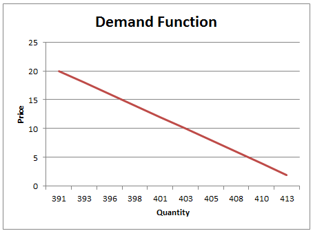
We will discuss some of the methods of estimating demand functions (or curves) given in previous part “Demand Analysis: Segment 2”.

1. Leontief’s Method (from Time Series Data)

Assumptions:

1. Each market transaction represents the intersection of instantaneous demand and supply curves which change their position periodically. This implies that in addition to determining the elasticity of both demand and supply, we must also study the extent to which the curves have shifted from time to time.
2. The shifting of demand and supply curves are independent of each other and do not affect the shape (elasticity) of the curves. This means that a shift of the demand curve to the right is just as likely to be associated with a shift of the supply curve to the left as to the right.
3. Each of the supply and demand curves is of constant elasticity, i.e., the demand and supply curves when plotted on a double logarithmic scale should be straight lines.

Limitations: Leontief’s method has a number of economic and statistical objections (limitations):

1. The assumption that Cournot-Marshall demand and supply curves can shift in any direction, and that the shifting of the two curves are independent of each other violates the fundamental principle of the general theory of equilibrium viz., “the demand of any one commodity is a function not only of its price but also of all other prices.”
2. Leontief’s assumption that the supply and demand curves shift simultaneously is not a reasonable assumption for agricultural commodity. For example, a high (low) price for a commodity in any one year is, on the average, associated with a high (low) production of the commodity in the following year.
3. The assumption that elasticity of both demand and supply are constant may not hold.

1. Pigous’ Method (from Time Series Data)

Assumptions:

1. The demand curve is likely to have a smooth appearance in each interval, i.e., the demand curve, for each interval of time, is a curve of constant elasticity.
2. The demand curve shifts steadily over different periods of time, the rate of shifts being equal in two successive intervals. In other words, Pigous assumed that the rate of shift is such that the distance between the i^th and (i+1)^th position (on a logarithmic scale) is same as the distance between (i+1)^th and (i+2)^th position.

Limitations:

1. Pigous’ method is based on the assumption that the demand curve for the commodity may be written as:

x=f(p,t)

where ‘x’ is the quality of the commodity that is demanded, ‘p’ is the price of the commodity demanded and ‘t’ is time. This implicitly assumes that the prices of all other related commodities have only a negligible or no effect upon the commodity in question or all the influencing factors are conceived as frozen while studying the variations in ‘x’ as a result of variations in ‘y’. However, in practice it is impossible to freeze all other factors without first taking them into account.

1. The method breaks down completely if in the three successive sets of observations, the three price-quantity points are collinear. Therefore, practically the method will fail if the successive observations are almost collinear. However, the method can be applied to non-linear functions and the functions which change in directions.
2. It is not applicable to those cases, where the underlying theoretical curve of demand changes its direction of motion.

Click here for government certification in Statistics and Quality