Probabilistic Distributions- Probability distributions are a fundamental concept in statistics. They are used both on a theoretical level and a practical level.
Some practical uses of probability distributions are:
- To calculate confidence intervals for parameters and to calculate critical regions for hypothesis tests.
- For univariate data, it is often useful to determine a reasonable distributional model for the data.
- Statistical intervals and hypothesis tests are often based on specific distributional assumptions. Before computing an interval or test based on a distributional assumption, we need to verify that the assumption is justified for the given data set. In this case, the distribution does not need to be the best-fitting distribution for the data, but an adequate enough model so that the statistical technique yields valid conclusions.
- Simulation studies with random numbers generated from using a specific probability distribution are often needed.
With probability, statements are made about the chances that certain outcomes will occur, based on an assumed model. With statistics, observed data is used to determine a model that describes this data. This model relates to the distribution of the data. Statistics moves from the sample to the population while probability moves from the population to the sample.
Inferential statistics is the science of describing population parameters based on sample data. Inferential statistics can be used to:
- Establish a process capability (determine defects per million).
- Utilize distributions to estimate the probability of a variable occurring given known parameters.
Inferential statistics are based on a normal distribution.
Figure 1: Normal Curve and Probability Areas
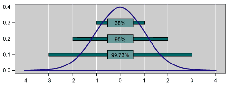
Normal curve distribution can be expanded on to learn about other distributions. The appropriate distribution can be assigned based on an understanding of the process being studied in conjunction with the type of data being collected and the dispersion or shape of the distribution. It can assist with determining the best analysis to perform.
Types of Distributions
Distributions are classified in the same ways as data is classified – continuous and discrete:
- Continuous probability distributions are probabilities associated with random variables that are able to assume any of an infinite number of values along an interval.
- Discrete probability distributions are listings of all possible outcomes of an experiment, along with their respective probabilities of occurrence.
Distribution Descriptions
Probability mass function (pmf) – For discrete variables, the pmf is the probability that a variate takes the value x.
Probability density function (pdf) – For continuous variables, the pdf is the probability that a variate assumes the value x, expressed in terms of an integral between two points.
In the continuous sense, one cannot give a probability of a specific x on a continuum – it will be some specific (and small) range. For additional insight, think of x + Dx where Dx is small.
The notation for the pdf is f(x). For discrete distributions:
f(x) = P(X = x)
Some refer to this as the probability mass function, since it is evaluating the probability upon that one discrete mass. For continuous distributions, one mass cannot be established.
Cumulative density function (cdf) – The probability that a variable takes a value less than or equal to x.
Figure 2: Normal Distribution Cdf
Cdf progresses to a value of 1 because there cannot be a probability greater than 1. Once again, cdf is F(x) = P(X < x).This holds for both continuous and discrete.
Parameters
Parameter is a population description. Consultants rely on parameters to characterize the distributions. There are three parameters:
- Location parameter – the lower or midpoint (as prescribed by the distribution) of the range of the variate (think of the mean)
- Scale parameter – determines the scale of measurement for x (magnitude of the x-axis scale) (think of the standard deviation)
- Shape parameter – defines the pdf shape within a family of shapes
Not all distributions have all the parameters. For example, the normal distribution parameters have just the mean and standard deviation. Just those two need to be known to describe a normal population.
Summary of Distributions
The remaining portion of this article will summarize the various shapes, basic assumptions and uses of distributions. Keep in mind that there is a different pdf and different distribution parameters associated with each.
Normal Distribution (Gaussian Distribution)
Figure 3: Normal Distribution Shape
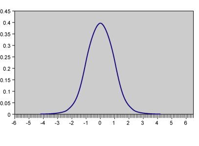
Basic assumptions:
- Symmetrical distribution about the mean (bell-shaped curve)
- Commonly used in inferential statistics
- Family of distributions characterized is by m and s
Uses include:
- Probabilistic assessments of distribution of time between independent events occurring at a constant rate
- Mean is the inverse of the Poisson distribution
- Shape can be used to describe failure rates that are constant as a function of usage
Exponential Distribution
Figure 4:Exponential Distribution Shape
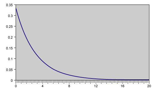
Basic assumptions:
- Family of distributions characterized by its m
- Distribution of time between independent events occurring at a constant rate
- Mean is the inverse of the Poisson distribution
- Shape can be used to describe failure rates that are constant as a function of usage
Uses include probabilistic assessments of:
- Mean time between failure (MTBF)
- Arrival times
- Time, distance or space between occurrences of the events of interest
- Queuing or wait-line theories
Lognormal Distribution
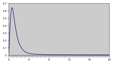
Figure 5: Lognormal Distribution Shape
Basic assumptions:
Asymmetrical and positively skewed distribution that is constrained by zero.
- Distribution can exhibit many pdf shapes
- Describes data that has a large range of values
- Can be characterized by m and s
Uses include simulations of:
- Distribution of wealth
- Machine downtimes
- Duration of time
- Phenomenon that has a positive skew (tails to the right)
Weibull Distribution
Figure 6: Weibull Distribution Pdf

Basic assumptions:
- Family of distributions
- Can be used to describe many types of data
- Fits many common distributions (normal, exponential and lognormal)
- The differing factors are the scale and shape parameters
Uses include:
- Lifetime distributions
- Reliability applications
- Failure probabilities that vary over time
- Can describe burn-in, random, and wear-out phases of a life cycle (bathtub curve)
Binomial Distribution
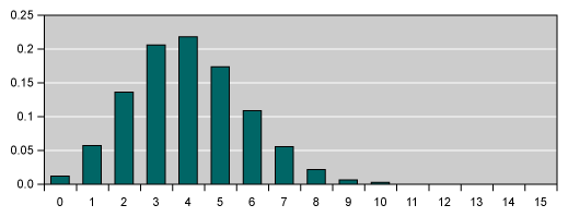
Figure 7: Binomial Distribution Shape
Basic assumptions:
- Discrete distribution
- Number of trials are fixed in advance
- Just two outcomes for each trial
- Trials are independent
- All trials have the same probability of occurrence
Uses include:
- Estimating the probabilities of an outcome in any set of success or failure trials
- Sampling for attributes (acceptance sampling)
- Number of defective items in a batch size of n
- Number of items in a batch
- Number of items demanded from an inventory
Geometric
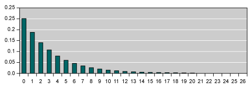
Figure 8: Geometric Distribution Pdf
Basic assumptions:
- Discrete distribution
- Just two outcomes for each trial
- Trials are independent
- All trials have the same probability of occurrence
- Waiting time until the first occurrence
Uses include:
- Number of failures before the first success in a sequence of trials with probability of success p for each trial
- Number of items inspected before finding the first defective item – for example, the number of interviews performed before finding the first acceptable candidate
Negative Binomial
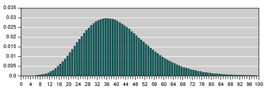
Figure 9: Negative Binomial Distribution Pdf
Basic assumptions:
- Discrete distribution
- Predetermined number of occurrences – s
- Just two outcomes for each trial
- Trials are independent
- All trials have the same probability of occurrence
Uses include:
- Number of failures before the sth success in a sequence of trials with probability of success p for each trial
- Number of good items inspected before finding the sth defective item
Poisson Distribution
Figure 10: Poisson Distribution Pdf
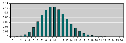
Basic assumptions:
- Discrete distribution
- Length of the observation period (or area) is fixed in advance
- Events occurs at a constant average rate
- Occurrences are independent
- Rare event
Uses include:
- Number of events in an interval of time (or area) when the events are occurring at a constant rate
- Number of items in a batch of random size
- Design reliability tests where the failure rate is considered to be constant as a function of usage
Hypergeometric
Shape is similar to Binomial/Poisson distribution.
Basic assumptions:
- Discrete distribution
- Number of trials are fixed in advance
- Just two outcomes for each trial
- Trials are independent
- Sampling without replacement
- This is an exact distribution – the Binomial and Poisson are approximations to this
Other Distributions
There are other distributions – for example, sampling distributions and X2, t and F distributions.
Test Your Six Sigma Black Belt Skills By Taking Our Practice Tests on This Link
Apply for Six Sigma Black Belt Certification Now!!
http://www.vskills.in/certification/Certified-Six-Sigma-Black-Belt-Professional


