Correlation is tool that is with a continuous x and a continuous y. Correlation begins with investigating the relationship between x factors, inputs, and critical variable y outputs of the process. It involves addressing the following questions like Does a relationship exist? or How strong is that relationship? or Which of those x inputs have the biggest impact or relationship to your y factors? What’s the hierarchy of importance that you’re going to need to pursue later in the improvement process?
Correlation doesn’t specifically look for causes and effects. It focuses only on whether there is a correlation between the x factors, y factors, and how strong that relationship is to the y variable output in your business process. The correlation between two variables does not imply that one is as a result of the other. The correlation value ranges from -1 to 1. The closer to value 1 signify positive relationship with x and y going in same direction similarly if nearing -1, both are in opposite direction and zero value means no relationship between the x and y.
Correlation analysis starts with relating the x inputs to the continuous y variable outputs. You do this over a range of observations, in which the x values and inputs can change over time. By doing this, you’re able to identify and begin to understand the key x inputs to the processes and the relationship between different x outputs.
Often the interaction of these different x factors can be a real challenge to understand in Six Sigma projects. A specific methodology called design of experiments defines a rigorous set of steps for identifying the various x factors, the variable y output factors, setting up and staging series of experiments to compare multiple x factors to one another, and their impact on the y, based on their interactions. So there are some powerful tools that enable you to go beyond just basic once-off x-factor analysis.
In product companies, for example, in circuit board assembly operations, you may be interested in knowing the number of hours of experience of the workers and comparing and correlating that to the percentage of incorrectly installed circuit modules. You might want to do visual acuity tests and determine if the visual acuity of your workers correlates to incorrectly installed modules on the circuit boards.
In service companies, for example, you may want to know about the correlation of blood pressure to the relative age of patients. When considering sales, you might want to know if you can correlate sales volume achieved to level of education and number of years of experience in the industry that you’re selling in. You may not get a causation but you could show a strong correlation that would lead you to further discoveries.
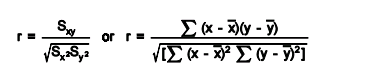
Measure of correlation – The correlation coefficient is a measure that determines the degree to which two variables’ movements are associated. The range of values for the correlation coefficient is -1.0 to 1.0. If a calculated correlation is greater than 1.0 or less than -1.0, a mistake has been made. A correlation of -1.0 indicates a perfect negative correlation, while a correlation of 1.0 indicates a perfect positive correlation.
While the correlation coefficient measures a degree to which two variables are related, it only measures the linear relationship between the variables. Nonlinear relationships between two variables cannot be captured or expressed by the correlation coefficient. There are many measures of correlation. The Pearson correlation coefficient is just one of them.
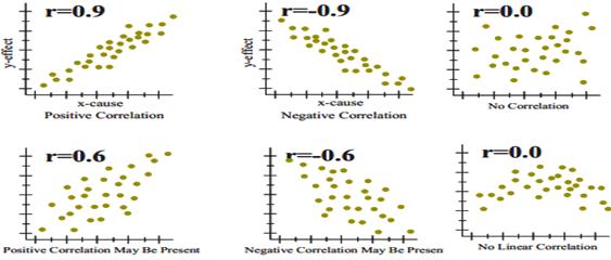
To gain an understanding of correlation coefficients, consider how the scatter diagrams would differ for different coefficient values:
- with a correlation coefficient value of 1, plotted data points would form a straight line that rises from left to right
- with a correlation coefficient value of 0.82, the plotted data would maintain a similar line, but the data points would be more loosely scattered on either side of it
- with a correlation coefficient value of 0, data points would be scattered widely and there would be no line of best fit
- with a correlation coefficient value of -0.67, the data points would be scattered to either side of a best-fit line that would slope downward from left to right
- with a correlation coefficient value of -1, the data points would form a straight line that would slope down from left to right
Confidence in a relationship is computed both by the correlation coefficient and by the number of pairs in data. If there are very few pairs then the coefficient needs to be very close to 1 or –1 for it to be deemed ‘statistically significant’, but if there are many pairs then a coefficient closer to 0 can still be considered ‘highly significant’. The standard method used to measure the ‘significance’ of analysis is the p-value. It is computed as
For example to know the relationship between height and intelligence of people is significant, it starts with the ‘null hypothesis’ which is a statement ‘height and intelligence of people are unrelated’. The p-value is a number between 0 and 1 representing the probability that this data would have arisen if the null hypothesis were true. In medical trials the null hypothesis is typically of the form that the use of drug X to treat disease Y is no better than not using any drug. The p-value is the probability of obtaining a test statistic result at least as extreme as the one that was actually observed, assuming that the null hypothesis is true. Project team usually “reject the null hypothesis” when the p-value turns out to be less than a certain significance level, often 0.05. The formula to calculate the p value for Pearson’s correlation coefficient (r) is p=r/Sqrt(r^2)/(N—2).
The Pearson coefficient is an expression of the linear relationship in data. It gives you a correlation expressed as a simple numerical value between -1 and 1. The Pearson coefficient can help you understand weaknesses. Weaknesses occur where you can’t distinguish between dependent and the independent variables, and there’s no information about the slope of the line. However, this coefficient may not tell you everything you want to know. For example, say you’re trying to find the correlation between a high-calorie diet, which is the dependent variable or cause, and diabetes, which is the independent variable or effect. You might find a high correlation between these two variables. However, the result would be exactly the same if you switch the variables around, which could lead you to conclude that diabetes causes a high-calorie diet. Therefore, as a researcher, you have to be aware of the context of the data that you’re plugging into your model.
