Arbitrage Pricing Theory (APT)

Certify and Increase Opportunity.
Be
Govt. Certified -Equity Research Analyst

Arbitrage Pricing Theory (APT)

5.6.1 Model Characteristics

APT, which stands for Arbitrage Pricing Theory, it is a asset pricing tool used to determine the expected returns of a stock, security or other type of investment. This theory was first proposed by Stephen Ross in 1976.

It is a multifactor approach to explain the pricing of asset. Ross developed a mechanism that derives asset prices from arbitrage arguments similar to but more complex than those used in CAPM. This is based on the law of one price: two items which are same cannot sell at different prices.

The APT description of equilibrium is more general than that provided by CAPM in that pricing can be affected by influences beyond simply means and variances. The assumption of homogenous expectations is necessary. The assumption of investors utilizing a mean variance framework is replaced by an assumption of the process generating security returns. The general idea behind APT is that two things can explain the expected return on a financial asset.

• Macro-economic and security-specific influences,
• The asset’s sensitivity to those influences.

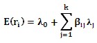
This relationship takes the following form of the linear regression formula:

Where:

= expected rate of return the  asset

= the risk-free rate of return

=  the sensitivity of the asset’s return to the factor

 = the risk premium associated with the

There are an infinite number of security-specific influences for any given security including inflation, production measures, investor confidence, exchange rates, market indices, or changes in interest rates. It is up to the analyst to decide which influences are relevant to the asset being analyzed.

APT can be applied to portfolios as well as individual securities since a portfolio can have exposures and sensitivities to certain kinds of risk factors as well. The APT was a revolutionary model because it allows the user to adapt the model to the security being analyzed. Like other pricing models, it helps the user decide whether a security is undervalued or overvalued and so that he or she can profit from this information. APT is also very useful for building portfolios because it allows managers to test whether their portfolios are exposed to certain factors.

APT may be more customizable than CAPM, but it is also more difficult to apply because determining which factors influence a stock or portfolio takes a considerable amount of research. It can be virtually impossible to detect every influential factor much less determine how sensitive the security is to a particular factor. But getting “close enough” is often good enough; in fact studies find that four or five factors will usually explain most of a security’s return: surprises in inflation, GNP, investor confidence, and shifts in the yield curve.

APT Models

The two most widely used APT models are.

• Fama French Model (FF model)
• Burmeister, Ibbotson, Roll & Ross model (BIRR model)

Fama French Model (FF model)

Fama and French (1993) presented the Fama and French Three Factors Model after their study revealed that the cross section of average stock returns for the period1963-1990 for US stocks is not fully explained by the CAPM beta and that stock risks are multidimensional.

They developed the pricing model that combined the following factors to explain the average return of stock;

• Market (Market risk premium),
• Size (Return of Small Size minus Return of Big Size: SMB ), and
• Book to Market Ratio: BE/ME Ratio (Return of High BE/ME Ratio minus Return of Low BE/ME Ratio): HML).

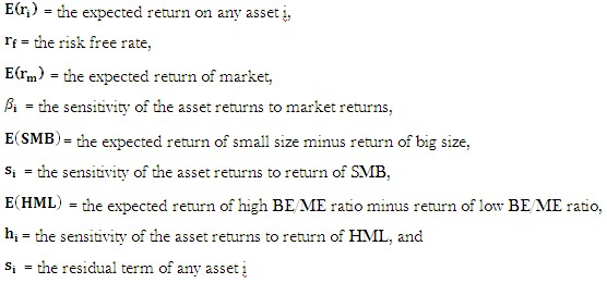
The Fama and French Three Factors Model equation is:

Where:

To create portfolios that track the firm size and book-to-market factors, Fama and French sorted industrial firms annually by size (market capitalization) and by book-to-market (B/M) ratio. The small-firm group (S) includes all firms with capitalization below the median. The big-firm group (B) has firms with above median capitalization.

Similarly, firms are annually sorted into three groups based on book-to-market ratio.

A low-ratio group (group L) is the one with the 33% lowest B/M ratio; a medium ratio group (group M), and a high-ratio group (group H). The high-ratio firms are called value firms, the low-ratio firms are called growth firms.

Burmeister, Ibbotson, Roll & Ross model (BIRR model) 

BIRR stands for Burmeister, Ibbotson, Roll and Ross. The BIRR model consists of five macroeconomic factors which are.

• Confidence Risk: Confidence Risk exposure reflects a stock’s sensitivity to unexpected changes in investor confidence. Investors always demand a higher return for making relatively riskier investments. When their confidence is high, they are willing to accept a smaller reward than when their confidence is low. Most assets have a positive exposure to Confidence Risk. An unexpected increase in investor confidence will put more investors in the market for these stocks, increasing their price and producing a positive return for those who already held them. Similarly, a drop in investor confidence leads to a drop in the value of these investments. Some stocks have a negative exposure to the Confidence Risk factor, however, suggesting that investors tend to treat them as a ‘safe haven’ when their confidence is shaken.

• Time Horizon Risk: The Time Horizon Risk exposure reflects a stock’s sensitivity to unexpected changes in investor’s willingness to invest for the long term. An increase in Time Horizon tends to benefit growth stocks, while a decrease tends to benefit income stocks. Exposures can be positive or negative, but growth stocks as a rule have a higher (more positive) exposure than income stocks.

• Inflation Risk: Inflation Risk exposure reflects a stock’s sensitivity to unexpected changes in the inflation rate. Unexpected increases in the inflation rate put a downward pressure on stock prices, so most stocks have a negative exposure to Inflation Risk. Consumer demand for luxuries declines when real income is eroded by inflation.Thus, retailers, eating places, hotels, resorts, and other ‘luxuries’ are harmed by inflation, and their stocks therefore tend to be more sensitive to inflation surprises and, as a result, have a more negative exposure to Inflation Risk. Conversely, providers of necessary goods and services (agricultural products, tire and rubber goods, etc.) are relatively less harmed by inflation surprises, and their stocks have a smaller (less negative) exposure. A few stocks attract investors in times of inflation surprise and have a positive Inflation Risk exposure.

• Business Cycle Risk: Business Cycle Risk exposure reflects a stock’s sensitivity to unexpected changes in the growth rate of business activity. Stocks of companies such as retail stores that do well in times of economic growth have a higher exposure to Business Cycle Risk than those that are less affected by the business cycle, such as utilities or government contractors. Stocks can have a negative exposure to this factor if investors tend to shift their funds toward those stocks when news about the growth rate for the economy is not good.

• Market Timing Risk: Market Timing Risk exposure reflects a stock’s sensitivity to moves in the stock market as a whole that cannot be attributed to the other factors. Sensitivity to this factor provides information similar to that of the CAPM beta about how a stock tends to respond to changes in the broad market. It differs in that the Market Timing Risk factor reflects only those surprises that are not explained by the other four factors. Using the linear factor model assumptions and the pricing equation is as follows.

Where:

  = The risk free-free rate is

= The price of risk or risk premium for the corresponding risk factor.

CAPM vs. APT

Capital asset pricing model (CAPM) and arbitrage pricing theory (APT) are both asset pricing models for assessing an investment’s risk in relation to its potential rewards. Essentially, they both use formulae to determine what kind of return an investment needs to yield in order to make it worthwhile. In both the models the investor compares the investment’s risks and returns with other investments’ risks and returns.

The comparison of the two models can be summarized as follows.

Formula

• CAPM’s formula is: Expected rate of return= risk-free rate + beta x (expected overall market return – risk-free rate).
• APT’s formula is: Expected rate of return = risk-free rate + (individual factor) x (relationship between price and the factor) + (individual factor) x (relationship between price and the factor) +….+ up to nth factor

The similarities, then, are the presence of the risk-free rate.

Risk factors

• The CAPM model uses a beta factor, which is riskiness of the stock in relation to the market as a whole. If it is risky as the stock market, it would be 1, if it is twice as risky, it would be 2, and so on. APT, on the other hand, uses individual factors, which change depending on the stock.

Rates of return

• CAPM uses the whole market’s rate of return while APT does not.

This indicates that an APT formula is more specific to that stock while the CAPM formula is more in terms of what may be earned elsewhere.

Objectivity

• CAPM uses a lot of objective data that is widely available. APT, on the other hand, uses data that is specific to that stock. Theoretically this is superior, but in practice it is difficult to determine which data is important and which data is not, and to what extent it has influence. So, APT is more helpful when it is used correctly, but CAPM is simpler.